Transcription
Deconfounded Lexicon Inductionfor Interpretable Social ScienceReid Pryzant , Kelly Shen , Dan Jurafsky † , Stefan Wager‡ Department of Computer Science†Department of Linguistics‡Graduate School of BusinessStanford ord.eduAbstractNLP algorithms are increasingly used in computational social science to take linguistic observations and predict outcomes like humanpreferences or actions. Making these socialmodels transparent and interpretable often requires identifying features in the input that predict outcomes while also controlling for potential confounds. We formalize this need asa new task: inducing a lexicon that is predictive of a set of target variables yet uncorrelated to a set of confounding variables. Weintroduce two deep learning algorithms for thetask. The first uses a bifurcated architectureto separate the explanatory power of the textand confounds. The second uses an adversarialdiscriminator to force confound-invariant textencodings. Both elicit lexicons from learnedweights and attentional scores. We use themto induce lexicons that are predictive of timelyresponses to consumer complaints (controllingfor product), enrollment from course descriptions (controlling for subject), and sales fromproduct descriptions (controlling for seller).In each domain our algorithms pick wordsthat are associated with narrative persuasion;more predictive and less confound-related thanthose of standard feature weighting and lexicon induction techniques like regression andlog odds.1IntroductionApplications of NLP to computational social science and data science increasingly use lexical features (words, prefixes, etc) to help predict nonlinguistic outcomes like sales, stock prices, hospital readmissions, and other human actions or preferences. Lexical features are useful beyond predictive performance. They enhance interpretability in machine learning because practitioners knowwhy their system works. Lexical features can alsobe used to understand the subjective properties ofa text.For social models, we need to be able to selectlexical features that predict the desired outcome(s)while also controlling for potential confounders.For example, we might want to know which wordsin a product description lead to greater sales, regardless of the item’s price. Words in a descriptionlike “luxury” or “bargain” might increase salesbut also interact with our confound (price). Suchwords don’t reflect the unique part of text’s effect on sales and should not be selected. Similarly, we might want to know which words in aconsumer complaint lead to speedy administrativeaction, regardless of the product being complainedabout; which words in a course description lead tohigher student enrollment, regardless of the coursetopic. These instances are associated with narrative persuasion: language that is responsible foraltering cognitive responses or attitudes (Spence,1983; Van Laer et al., 2013).In general, we want words which are predictiveof their targets yet decorrelated from confounding information. The lexicons constituted by thesewords are useful in their own right (to developcausal domain theories or for linguistic analysis)but also as interpretable features for down-streammodeling. Such work could help widely in applications of NLP to tasks like linking text to salesfigures (Ho and Wu, 1999), to voter preference(Luntz, 2007; Ansolabehere and Iyengar, 1995), tomoral belief (Giles et al., 2008; Keele et al., 2009),to police respect (Voigt et al., 2017), to financialoutlooks (Grinblatt and Keloharju, 2001; Chatelain and Ralf, 2012), to stock prices (Lee et al.,2014), and even to restaurant health inspections(Kang et al., 2013).Identifying linguistic features that are indicativeof such outcomes and decorrelated with confoundsis a common activity among social scientists, datascientists, and other machine learning practitioners. Indeed, it is essential for developing transpar-
ent and interpretable machine learning NLP models. Yet there is no generally accepted and rigorously evaluated procedure for the activity. Practitioners have conducted it on a largely ad-hocbasis, applying various forms of logistic and linear regression, confound-matching, or associationquantifiers like mutual information or log-odds toachieve their aims, all of which have known drawbacks (Imai and Kim, 2016; Gelman and Loken,2014; Wurm and Fisicaro, 2014; Estévez et al.,2009; Szumilas, 2010).We propose to overcome these drawbacks viatwo new algorithms that consider the causal structure of the problem. The first uses its architecture to learn the part of the text’s effect whichthe confounds cannot explain. The second usesan adversarial objective function to match text encoding distributions regardless of confound treatment. Both elicit lexicons by considering learnedweights or attentional scores. In summary, we1. Formalize the problem into a new task.2. Propose a pair of well-performing neural network based algorithms.3. Conduct the first systematic comparison ofalgorithms in the space, spanning three domains: consumer complaints, course enrollments, and e-commerce product descriptions.The techniques presented in this paper will helpscientists (1) better interpret the relationship between words and real-world phenomena, and (2)render their NLP models more interpretable1 .2Deconfounded Lexicon InductionWe begin by formalizing this language processingactivity into a task. We have access to text(s) T ,target variable(s) Y , and confounding variable(s)C. The goal is to pick a lexicon L such that whenwords in T belonging to L are selected, the resulting set L(T ) is related to Y but not C. Thereare two types of signal at play: the part of Y thatT can explain, and that explainable by C. Thesesignals often overlap because language reflects circumstance, but we are interested in the part of T ’sexplanatory power which is unique to T , and hopeto choose L accordingly.So if Var [E [Y L(T ), C]] is the information inY explainable by both L(T ) and C, then our goal1Code, hyperparameters, and instructions for practitioners are online at icon-induction/is to choose L such that this variance is maximizedafter C has been fixed. With this in mind, we formalize the task of deconfounded lexicon induction as finding a lexicon L that maximizes aninformativeness coefficient, I(L) E Var E Y L(T ), C C ,(1)which measures the explanatory power of the lexicon beyond the information already contained inthe confounders C. Thus, highly informative lexicons cannot simply collect words that reflect theconfounds. Importantly, this coefficient is onlyvalid for comparing different lexicons of the samesize, because in terms of maximizing this criterion,using the entire text will trivially make for the bestpossible lexicon.Our coefficient I(L) can also be motivated viaconnections to the causal inference literature: inSection 7, we show that—under assumptions often used to analyze causal effects in observationalstudies—the coefficient I(L) can correspond exactly to the strength of T ’s causal effects on Y .Finally, note that by expanding out an ANOVAdecomposition for Y , we can re-write this criterionash 2 iI(L) E Y E Y C, L(T )h(2) 2 i , E Y E Y Ci.e., I(L) measures the performance improvementL(T ) affords to optimal predictive models that already have access to C. We use this fact for evaluation in Section 4.3Proposed AlgorithmsWe continue by describing the pair of novel algorithms we are proposing for deconfounded lexiconinduction problems.3.1Deep Residualization (DR)Motivation. Our first method is directly motivatedby the setup from Section 2. Recall that I(L)measures the amount by which L(T ) can improvepredictions of Y made from the confounders C.We accordingly build a neural network architecture that first predicts Y directly from C as well aspossible, and then seeks to fine-tune those predictions using T .Description. First we pass the confounds througha feed-forward neural network (FFNN) to obtain
(FFNN):t [f req1 , f req2 , ., f reqk ]h ReLU (W hidden t)e ReLU (W output t)We then concatenate e with Ŷ 0 and feed the result through another neural network to generate final predictions Ŷ . If Y is continuous we computeloss withLcontinuous Ŷ Y 2If Y is categorical we compute loss withFigure 1: The Deep Residualization (DR) selector. Values which are used to calculate losses are enclosed inred ovals. Top: DR ATTN, which represents text asa sequence of word embeddings. Bottom: DR BOW,which represents text as a vector of word frequencies.preliminary predictions Ŷ 0 . We also encode thetext into a continuous vector e Rd via two alternative mechanisms:1. DR ATTN: the text is converted into asequence of embeddings and fed intoLong Short-Term Memory (LSTM) cell(s)(Hochreiter and Schmidhuber, 1997) followed by an attention mechanism inspiredby Bahdanau et al. (2015). If the wordsof a text have been embedded as vectorsx1 , x2 , ., xn then e is calculated as aweighted average of hidden states, where theweights are decided by a FFNN whose parameters are shared across timesteps:h0 0ht LST M (xt , ht 1 )lt ReLU (W attn ht ) · v attnexp(lt )pt Pexp(li )Xe pi hi2. DR BOW: the text is converted into a vector of word frequencies, which is compressedwith a two-layer feedforward neural networkLcategorical p log pb Where pb corresponds to the predicted probabilityof the correct class. The errors from Ŷ are propagated through the whole model, but the errors fromŶ 0 are only used to train its progenitor (Figure 1).Note the similarities between this model and thepopular residualizing regression (RR) technique(Jaeger et al., 2009; Baayen et al., 2010, inter alia).Both use the text to improve an estimate generated from the confounds. RR treats this as twoseparate regression tasks, by regressing the confounds against the variables of interest, and thenusing the residuals as features, while our modelintroduces the capacity for nonlinear interactionsby backpropagating between RR’s steps.Lexicon Induction. We elicit lexicons from ATTN style models by (1) running inference ona test set, but rather than saving those predictions,saving the attentional distribution over each sourcetext, and (2) mapping each word to its average attentional score and selecting the k highest-scoringwords.For BOW style models, we take the matrix thatcompresses the text’s word frequency vector, thenscore each word by computing the l1 norm of thecolumn that multiplies it, with the intuition thatimportant words are dotted with big vectors in order to be a large component of e.3.2Adversarial Selector (A)Motivation. We begin by observing that a desirable L can explain Y , but is unrelated to C, whichimplies it should should struggle to predict C. TheAdversarial Selector draws inspiration from this.
Figure 2: The Adversarial (A) selector. Values whichare used to calculate losses are enclosed in red ovals.Top: A ATTN, which represents text as a sequence ofword embeddings. Bottom: A BOW, which representstext as a vector of word frequencies.It learns adversarial encodings of T which are useful for predicting Y , but not useful for predictingC. It is depicted in Figure 2.Description. First, we encode T into e Rd viathe same mechanisms as the Deep Residualizer ofSection 3.1. e is then passed to a series of FFNNs(“prediction heads”) which are trained to predicteach target and confound with the same loss functions as that of Section 3.1. As gradients backpropagate from the confound prediction heads tothe encoder, we pass them through a gradient reversal layer in the style of Ganin et al. (2016) andBritz et al. (2017), which multiplies gradients by 1. If the cumulative loss of the target variablesis Lt and that of the confounds is Lc , then theloss which is implicitly used to train the encoderis Le Lt Lc , thereby encouraging the encoderto learn representations of the text which are notuseful for predicting the confounds.Lexicons are elicited from this model via thesame mechanism as the Deep Residualizer of Section 3.1.4ExperimentsWe evaluate the approaches described in Sections 3 and 5 by generating and evaluating deconfounded lexicons in three domains: financialcomplaints, e-commerce product descriptions, andcourse descriptions. In each case the goal isto find words which can always help someonenet a positive outcome (fulfillment, sales, enrollment), regardless of their situation. This involvesfinding words associated with narrative persuasion: predictive of human decisions or preferencesbut decorrelated from non-linguistic informationwhich could also explain things. We analyze theresulting lexicons, especially with respect to theclassic Aristotelian modes of persuasion: logos,pathos, and ethos.We compare the following algorithms:Regression (R), Regression with Confoundfeatures (RC), Mixed effects Regression (M),Residualizing Regressions (RR), Log-Odds Ratio(OR), Mutual Information (MI), and MI/OR withregresssion (R MI and R OR). See Section 5 fora discussion of these baselines, and the onlinesupplementary information for implementationdetails. We also compare the proposed algorithms:Deep Residualization using word frequencies(DR BOW) and embeddings (DR ATTN), andAdversarial Selection using word frequencies(A BOW) and embeddings (A ATTN).In Section 2 we observed that I(L) measuresthe improvement in predictive power that L(T ) affords a model already having access to C. Thus,we evaluate each algorithm by (1) regressing Con Y , (2) drawing a lexicon L, (3) regressingC L(T ) on Y , and (4) measuring the size ofgap in test prediction error between the models ofstep (1) and (3). For classification problems, wemeasured error with cross-entropy (XE):XXE pi log pˆiiperformance XEC XEL(T ),CAnd for regression, we computed the meansquared error (MSE):MSE 1X(Ŷi Yi )2niperformance MSEC MSEL(T ),CBecause we fix lexicon size but vary lexicon content, lexicons with good words will score highlyunder this metric, yielding the large performanceimprovements when combined with C.We also report the average strength of association between words in L and C. For categoricalconfounds, we measure Cramer’s V (V ) (Cramér,2016), and for continuous confounds, we use the
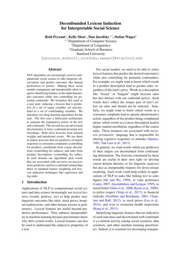
point-biserial correlation coefficient (rpb ) (Glassand Hopkins, 1970). Note that rpb is mathematically equivalent to Pearson correlation in bivariate settings. Here the best lexicons will score thelowest.We implemented neural models with the Tensorflow framework (Abadi et al., 2016) and optimized using Adam (Kingma and Ba, 2014). Weimplemented linear models with the scikit learnpackage (Pedregosa et al., 2011). We implementedmixed models with the lme4 R package (Bateset al., 2014). We refer to the online supplementarymaterials for per-experiment hyperparameters.For each dataset, we constructed vocabulariesfrom the 10,000 most frequently occurring tokens,and randomly selected 2,000 examples for evaluation. We then conducted a wide hyperparametersearch and used lexicon performance on the evaluation set to select final model parameters. We thenused these parameters to induce lexicons from 500random train/test splits. Significance is estimatedwith a bootstrap procedure: we counted the number of trials each algorithm “won” (i.e. had thelargest errorC errorL(T ),C ). We also reportthe average performance and correlation of all thelexicons generated from each split. We ran theseexperiments using lexicon sizes of k 50, 150,250, and 500 and observed similar behavior. Theresults reported in the following sections are fork 150, and the words in Tables 1, and 2, 3 arefrom randomly selected lexicons (other lexiconshad similar characteristics).4.1Consumer Financial Protection Bureau(CFPB) ComplaintsSetup. We consider 189,486 financial complaintspublicly filed with the Consumer Financial Protection Bureau (CFPB)2 . The CFPB is a productof Dodd-Frank legislation which solicits and addresses complaints from consumers regarding avariety of financial products: mortgages, credit reports, etc. Some submissions are handled on atimely basis ( 15 days) while others languish.We are interested in identifying salient wordswhich help push submissions through the bureaucracy and obtain timely responses, regardless ofthe specific nature of the complaint. Thus, ourtarget variable is a binary indicator of whetherthe complaint obtained a timely response. Our2These data can be obtained from umer-complaints/confounds are twofold, (1) a categorical variabletracking the type of issue (131 categories), and (2)a categorical variable tracking the financial product (18 categories). For the proposed DR BOW,DR ATTN, A BOW, and A ATTN models, weset e to 1, 64, 1, and 256, respectively.Results. In general, this seems to be a tractableclassification problem, and the confounds aloneare moderately predictive of timely response(XEC 1.06). The proposed methods appearto perform the best, and DR BOW achieved thelargest performance/correlation ratio (Figure 3).Figure 3: Predictive performance (XEC XEL(T ),C )and average confound correlation (V /rpb ) of lexiconsgenerated via our proposed algorithms and a variety ofmethods in current use. The numbers to the right ofeach bar indicate the number of winning bootstrap trials.DR owehipaafileacrossTable 1: The ten highest-scoring words in lexicons generated by Deep Residualization BOW (DR BOW),Mutual Information (MI), Residialized Regression(RR), and regression (R).
We obtain further evidence upon examiningthe lexicons selected by four representative algorithms: proposed (DR BOW), a well-performingbaseline (RR), and two naive baselines (R, MI)(Table 1). MI’s words appear unrelated to theconfounds, but don’t seem very persuasive, andour results corroborate this: these words failedto add predictive power over the confounds (Figure 3). On the opposite end of the spectrum, R’swords appear somewhat predictive of the timelyresponse, but are confound-related: they includethe FDCPA (Fair Debt Collection Practices Act)and HIPAA (Health Insurance Portability and Accountability Act), which are directly related to theconfound of financial product.The top-scoring words in RR’s lexicon includenumbers (“6”, “150.00”) and words that suggestthat the issue is ongoing (“being”, “starting”). Onthe other hand, the words of DR BOW draw onthe rhetorical devices of ethos by respecting thereader’s authority (“ma’am”, “honor”), and logosby suggesting that the writer has been proactiveabout solving the issue (“multiple”, “submitted”,“xx/xx/xxx”, “ago”). These are narrative qualitiesthat align with two of the persuasion literature’s“weapons of influence”: reciprocation and commitment (Kenrick et al., 2005). Several algorithmsimplicitly favored longer (presumably more detailed) complaints by selecting common punctuation.4.2University Course DescriptionsSetup. We consider 141,753 undergraduate andgraduate course offerings over a 6-year period(2010 - 2016) at Stanford University. We are interested in how the writing style of a descriptionconvinces students to enroll. We therefore chooselog(enrollment) as our target variable and controlfor non-linguistic information which students alsouse when making enrollment decisions: coursesubject (227 categories), course level (26), number of requirements satisfied (7), whether there isa final (3), the start time, and the combination ofdays the class meets (26). All except start time aremodeled as categorical variables. For the proposedDR BOW, DR ATTN, A BOW, and A ATTNmodels, we set e to 1, 100, 16, and 64, respectively.Results. This appears to be a tractable regressionproblem; the confounds alone are highly predictive of course enrollment (MSEC 3.67). (Fig-A ndTable 2: The ten highest-scoring words in lexicons generated by Adversarial ATTN (A ATTN), Regression(R), and Log-Odds Ratio (OR).ure 4). A ATTN performed the best, and in general, the proposed techniques produced the mostpredictive and least-correlated lexicons. Interestingly, Residualization (RR) and Regression withConfounds (RC) appear to outperform the DeepResidualization selector.In Table 2 we observe stark differences betweenthe highest-scoring words of a proposed technique(A ATTN) and two baselines with opposing characteristics (R, OR) (Table 2). Words chosen viaRegression (R) appear predictive of enrollment,but also related to the confounds of subject (“programming”, “computer”, “management”, “chemical”, “clinical”) and level (“required”, “prerequisites”, “introduction”).Figure 4:mance.Course description comparative perfor-Log-Odds Ratio (OR) selected words which
A izupolite suffixproteinpolite prefixgrainnutritionpolite ationtranslationnichibanadhesive heetchemicalminiTable 3: The ten highest-scoring words in lexicons generated by Adversarial Selection BOW (A BOW) andResidualization (RR).appear unrelated to both the confounds andenrollment. The Adversarial Selector (A ATTN)selected words which are both confounddecorrelated and predictive of enrollment. Itswords appeal to the concept of variety (“or”,“guest”), and to pathos, in the form of universalstudent interests (“future”, “eating”, “sexual”).Notably, the A ATTN words are also shorter(mean length of 6.2) than those of R (9.3) andOR (9.0), which coincides with intuition (studentsoften skim descriptions) and prior research (shortwords are known to be more persuasive in somesettings (Pratkanis et al., 1988)). The lexicon alsosuggests that students prefer courses with researchproject components (“research”, “project”).4.3eCommerce DescriptionsSetup. We consider 59,487 health product listingson the Japanese e-commerce website Rakuten3 .These data originate from a December 2012 snapshot of the Rakuten marketplace. They were tokenized with the JUMAN morphological analyzer(Kurohashi and Nagao, 1999).We are interested in identifying words whichadvertisers could use to increase their sales, regardless of the nature of the product. Therefore,we set log(sales) as our target variable, and control for an item’s price (continuous) and seller (207categories). The category of an item (i.e. toothbrush vs. supplement) is not included in thesedata. In practice, sellers specialize in particularproduct types, so this may be indirectly accountedfor. For the proposed DR BOW, DR ATTN,A BOW, and A ATTN models, we set e to 4,3These data can be obtained from https://rit.rakuten.co.jp/data release/Figure 5: E-commerce comparative performance.64, 4, and 30, respectively.Results. This appears to be a more difficult prediction task, and the confounds are only slightlypredictive of sales (MSEC 116.34) (Figure 5).Again, lexicons obtained via the proposed methods were the most successful, achieving the highest performance with the lowest correlation (Table 3). When comparing the words selected byA BOW (proposed) and RR (widely used andwell performing), we find that both draw on therhetorical element of logos and demonstrate informativeness (“nutrition”, “size”, etc.). A BOWalso draws on ethos by identifying word stems associated with politeness. This quality draws on theauthority of shared cultural values, and has beenshown to appeal to Japanese shoppers (Pryzantet al., 2017). On the other hand, RR selected sev-
eral numbers and failed to avoid brand indicators:“nichiban”, a large company which specializes inmedical adhesives, is one of the highest-scoringwords.5Related WorkThere are three areas of related work which wedraw on. We address these in turn.Lexicon induction. Some work in lexicon induction is intended to help interpret the subjectiveproperties of a text or make make machine learning models more interpretable, i.e. so that practitioners can know why their system works. Forexample, Taboada et al. (2011); Hamilton et al.(2016) induce sentiment lexicons, and Mohammad and Turney (2010); Hu et al. (2009) induceemotion lexicons. Practitioners often get thesewords by considering the high-scoring features ofregressions trained to predict an outcome (McFarland et al., 2013; Chahuneau et al., 2012; Ranganath et al., 2013; Kang et al., 2013). They account for confounds through manual inspection,residualizing (Jaeger et al., 2009; Baayen et al.,2010), hierarchical modeling (Bates, 2010; Gustarini, 2016; Schillebeeckx et al., 2016), log-odds(Szumilas, 2010; Monroe et al., 2008), mutual information (Berg, 2004), or matching (Tan et al.,2014; DiNardo, 2010). Many of these methodsare manual processes or have known limitations,mostly due to multicollinearity (Imai and Kim,2016; Chatelain and Ralf, 2012; Wurm and Fisicaro, 2014). Furthermore, these methods have notbeen tested in a comparative setting: this work isthe first to offer an experimental analysis of theirabilities.Causal inference. Our methods for lexicon induction have connections to recent advances in thecausal inference literature. In particular, Johansson et al. (2016) and Shalit et al. (2016) proposean algorithm for counterfactual inference whichbear similarities to our Adversarial Selector (Section 3.2), Imai et al. (2013) advocate a lasso-basedmethod related to our Deep Residualization (DR)method (Section 3.1), and Egami et al. (2017) explore how to make causal inferences from textthrough careful data splitting. Unlike us, these papers are largely unconcerned with the underlyingfeatures and algorithmic interpretability. Athey(2017) has a recent survey of machine learningproblems where causal modeling is important.Persuasion. Our experiments touch on the mech-anism of persuasion, which has been widely studied. Most of this prior work uses lexical, syntactic, discourse, and dialog interactive features (Staband Gurevych, 2014; Habernal and Gurevych,2016; Wei et al., 2016), power dynamics (Rosenthal and Mckeown, 2017; Moore, 2012), or diction(Wei et al., 2016) to study discourse persuasion asmanifested in argument. We study narrative persuasion as manifested in everyday decisions. Thisimportant mode of persuasion is understudied because researchers have struggled to isolate the “active ingredient” of persuasive narratives (Green,2008; De Graaf et al., 2012), a problem that theformal framework of deconfounded lexicon induction (Section 2) may help alleviate.6ConclusionComputational social scientists frequently developalgorithms to find words that are related to someinformation but not other information. We encoded this problem into a formal task, proposedtwo novel methods for it, and conducted the firstprincipled comparison of algorithms in the space.Our results suggest the proposed algorithms offer better performance than those which are currently in use. Upon linguistic analysis, we alsofind the proposed algorithms’ words better reflectthe classic Aristotelian modes of persuasion: logos, pathos, and ethos.This is a promising new direction for NLP research, one that we hope will help computational(and non-computational!) social scientists betterinterpret linguistic variables and their relation tooutcomes. There are many directions for futurework. This includes algorithmic innovation, theoretical bounds for performance, and investigating rich social questions with these powerful newtechniques.7Appendix: Causal Interpretation of theInformativeness CoefficientRecall the definition of I(L): I(L) E Var E Y L(T ), C CHere, we discuss how under standard (albeitstrong) assumptions that are often made to identify causal effects in observational studies, we caninterpret I(L) with L(T ) T as a measure of thestrength of the text’s causal effect on Y .Following the potential outcomes model of Rubin (1974) we start by imagining potential out-
comes Y (t) corresponding to the outcome wewould have observed given text t for any possibletext t T ; then we actually observe Y Y (T ).With this formalism, the causal effect of the textis clear, e.g., the effect of using text t0 versus t issimply Y (t0 ) Y (t).Suppose that T , our observed text, takes onvalues in T with a distribution that dependson C. Let’s also assume that the observedtext T is independent of the potential outcomes{Y (t)}t T , conditioned on the confounders C(Rosenbaum and Rubin, 1983). So we knowwhat would happen with any given text, but don’tyet know which text will get selected (becauseT is a random variable). Now if we fix C andtherein Y (T ) (i.e. is any variance remainingE Var Y (T ) C, {Y (t)}t T 0) then the texthas a causal effect on Y .Now we assume that Y (t) fc (t) , meaning that the difference in effects of one text t relative to another text t0 is always the same givenfixed confounders. For example, in a bag of wordsmodel, this would imply that switching from usingthe word “eating” versus “homework” in a coursedescription would always have the same impact onenrollment (conditionally on confounders). Withthis assumptionin hand, then the causal effects of T , E Var Y (T ) C, {Y (t)}t T , matches I(L)as described in equation (1) (Imbens and Rubin,2015). In other words, given the same assumptionsoften made in observational studies, the informativeness coefficient of the full, uncompressed textin fact corresponds to the amount of variation in Ydue to the causal effects of
con induction techniques like regression and log odds. 1 Introduction Applications of NLP to computational social sci-ence and data science increasingly use lexical fea-tures (words, prefixes, etc) to help predict non-linguistic outcomes like sales, stock prices, hospi-t