WIXLIB

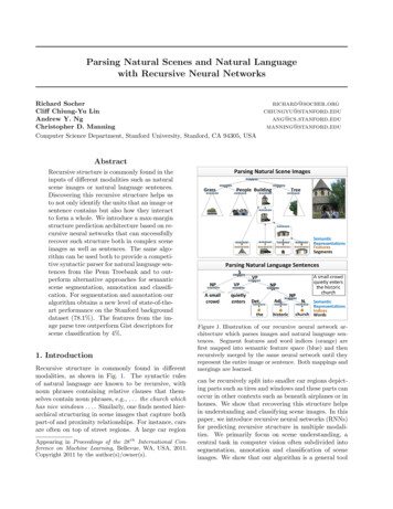
Parsing Natural Scenes and Natural Language with Recursive Neural NetworksDeep Learning in vision applications canfind lower dimensional representations for fixed sizeinput images which are useful for classification(Hinton & Salakhutdinov, 2006). Recently, Lee et al.(2009) were able to scale up deep networks to morerealistic image sizes. Using images of single objectswhich were all in roughly the same scale, they wereable to learn parts and classify the images into object categories. Our approach differs in several fundamental ways to any previous deep learning algorithm.(i) Instead of learning features from raw, or whitenedpixels, we use off-the-shelf vision features of segmentsobtained from oversegmented full scene images. (ii)Instead of building a hierarchy using a combination ofconvolutional and max-pooling layers, we recursivelyapply the same network to merged segments and giveeach of these a semantic category label. (iii) This isthe first deep learning work which learns full scene segmentation, annotation and classification. The objectsand scenes vary in scale, viewpoint, lighting etc.features for the segments as described in Sec. 3.1 of(Gould et al., 2009). These features include color andtexture features (Shotton et al., 2006), boosted pixelclassifier scores (trained on the labeled training data),as well as appearance and shape features.Using deep learning for NLP applications has beeninvestigated by several people (inter alia Bengio et al.,2003; Henderson, 2003; Collobert & Weston, 2008). Inmost cases, the inputs to the neural networks are modified to be of equal size either via convolutional andmax-pooling layers or looking only at a fixed size window around a specific word. Our approach is differentin that it handles variable sized sentences in a natural way and captures the recursive nature of natural language. Furthermore, it jointly learns parsingdecisions, categories for each phrase and phrase feature embeddings which capture the semantics of theirconstituents. In (Socher et al., 2010) we developed anNLP specific parsing algorithm based on RNNs. Thatalgorithm is a special case of the one developed in thispaper.In order to efficiently use neural networks inNLP, neural language models (Bengio et al., 2003;Collobert & Weston, 2008) map words to a vector representation. These representations are stored in aword embedding matrix L Rn V , where V is thesize of the vocabulary and n is the dimensionality ofthe semantic space. This matrix usually captures cooccurrence statistics and its values are learned. Assume we are given an ordered list of Nwords wordsfrom a sentence x. Each word i 1, . . . , Nwords hasan associated vocabulary index k into the columns ofthe embedding matrix. The operation to retrieve thei-th word’s semantic representation can be seen as asimple projection layer where we use a binary vector ekwhich is zero in all positions except at the k-th index,3. Mapping Segments and Words intoSyntactico-Semantic SpaceThis section contains an explanation of the inputs usedto describe scene images and natural language sentences and how they are mapped into the space inwhich the RNN operates.3.1. Input Representation of Scene ImagesWe closely follow the procedure described in(Gould et al., 2009) to compute image features.First, we oversegment an image x into superpixels (also called segments) using the algorithm from(Comaniciu & Meer, 2002). Instead of computingmultiple oversegmentations, we only choose one setof parameters. In our dataset, this results in an average of 78 segments per image. We compute 119Next, we use a simple neural network layer to mapthese features into the “semantic” n-dimensional spacein which the RNN operates. Let Fi be the featuresdescribed above for each segment i 1, . . . , Nsegs inan image. We then compute the representation:ai f (W sem Fi bsem ),(1)where W sem Rn 119 is the matrix of parameterswe want to learn, bsem is the bias and f is appliedelement-wise and can be any sigmoid-like function. Inour vision experiments, we use the original sigmoidfunction f (x) 1/(1 e x ).3.2. Input Representation for NaturalLanguage Sentencesai Lek Rn .(2)As with the image segments, the inputs are nowmapped to the semantic space of the RNN.4. Recursive Neural Networks forStructure PredictionIn our discriminative parsing architecture, the goal isto learn a function f : X Y, where Y is the set of allpossible binary parse trees. An input x consists of twoparts: (i) A set of activation vectors {a1 , . . . , aNsegs },which represent input elements such as image segmentsor words of a sentence. (ii) A symmetric adjacencymatrix A, where A(i, j) 1, if segment i neighborsj. This matrix defines which elements can be merged.For sentences, this matrix has a special form with 1’sonly on the first diagonal below and above the maindiagonal.

Parsing Natural Scenes and Natural Language with Recursive Neural Networksfollowing functions:fθ (x) arg max s(RNN(θ, x, ŷ)),(4)ŷ T (x)Figure 2. Illustration of the RNN training inputs: An adjacency matrix of image segments or words. A trainingimage (red and blue are differently labeled regions) definesa set of correct trees which is oblivious to the order inwhich segments with the same label are merged. See textfor details.We denote the set of all possible trees that can beconstructed from an input x as T (x). When trainingthe visual parser, we have labels l for all segments.Using these labels, we can define an equivalence set ofcorrect trees Y (x, l). A visual tree is correct if all adjacent segments that belong to the same class are mergedinto one super segment before merges occur with supersegments of different classes. This equivalence classover trees is oblivious to how object parts are internally merged or how complete, neighboring objects aremerged into the full scene image. For training the language parser, the set of correct trees only has one element, the annotated ground truth tree: Y (x) {y}.Fig. 2 illustrates this.4.1. Max-Margin EstimationSimilar to (Taskar et al., 2004), we define a structuredmargin loss (x, l, ŷ) for proposing a parse ŷ for input x with labels l. The loss increases when a segment merges with another one of a different label before merging with all its neighbors of the same label.We can formulate this by checking whether the subtree subT ree(d) underneath a nonterminal node d inŷ appears in any of the ground truth trees of Y (x, l): (x, l, ŷ) κ 1{subT ree(d) / Y (x, l)},(3)d N (ŷ)where N (ŷ) is the set of non-terminal nodes and κis a parameter. The loss of the language parseris the sum over incorrect spans in the tree, see(Manning & Schütze, 1999).Given the training set, we search for a function f withsmall expected loss on unseen inputs. We consider thewhere θ are all the parameters needed to compute ascore s with an RNN. The score of a tree y is high ifthe algorithm is confident that the structure of the treeis correct. Tree scoring with RNNs will be explainedin detail below. In the max-margin estimation framework (Taskar et al., 2004; Ratliff et al., 2007), we wantto ensure that the highest scoring tree is in the setof correct trees: fθ (xi ) Y (xi , li ) for all training instances (xi , li ), i 1, . . . , n. Furthermore, we want thescore of the highest scoring correct tree yi to be largerup to a margin defined by the loss . i, ŷ T (xi ):s(RNN(θ, xi , yi )) s(RNN(θ, xi , ŷ)) (xi , li , ŷ).These desiderata lead us to the following regularizedrisk function:J(θ) ri (θ) N1 λ(5)ri (θ) θ 2 , whereN i 12()max s(RNN(θ, xi , ŷ)) (xi , li , ŷ)ŷ T (xi )()s(RNN(θ, xi , yi ))maxyi Y (xi ,li )Minimizing this objective maximizes the correct tree’sscore and minimizes (up to a margin) the score of thehighest scoring but incorrect tree.Now that we defined the general learning framework,we will explain in detail how we predict parse treesand compute their scores with RNNs.4.2. Greedy Structure Predicting RNNsWe can now describe the RNN model that uses the activation vectors {a1 , . . . , aNsegs } and adjacency matrixA (as defined above) as inputs. There are more thanexponentially many possible parse trees and no efficient dynamic programming algorithms for our RNNsetting. Therefore, we find a greedy approximation.We start by explaining the feed-forward process on atest input.Using the adjacency matrix A, the algorithm finds thepairs of neighboring segments and adds their activations to a set of potential child node pairs:C {[ai , aj ] : A(i,j) 1}.(6)In the small toy image of Fig. 2, we would have the following pairs: {[a1 , a2 ], [a1 , a3 ], [a2 , a1 ], [a2 , a4 ], [a3 , a1 ],[a3 , a4 ], [a4 , a2 ], [a4 , a3 ], [a4 , a5 ], [a5 , a4 ]}. Each pair ofactivations is concatenated and given as input to a

Parsing Natural Scenes and Natural Language with Recursive Neural Networksof the tree. The final score that we need for structureprediction is simply the sum of all the local decisions: s(RNN(θ, xi , ŷ)) sd .(11)s W score p(9)p f (W [c1 ; c2 ] b)d N (ŷ)Figure 3. One recursive neural network which is replicatedfor each pair of possible input vectors. This network isdifferent to the original RNN formulation in that it predictsa score for being a correct merging decision.neural network. The network computes the potentialparent representation for these possible child nodes:p(i,j) f (W [ci ; cj ] b).(7)With this representation we can compute a localscore using a simple inner product with a row vectorW score R1 n :s(i,j) W score p(i,j) .(8)The network performing these functions is illustratedin Fig. 3. Training will aim to increase scores ofgood segment pairs (with the same label) and decreasescores of pairs with different labels, unless no moregood pairs are left.After computing the scores for all pairs of neighboringsegments, the algorithm selects the pair which receivedthe highest score. Let the score sij be the highestscore; we then (i) Remove [ai , aj ] from C, as well asall other pairs with either ai or aj in them. (ii) Updatethe adjacency matrix with a new row and column thatreflects that the new segment has the neighbors of bothchild segments. (iii) Add potential new child pairs toC:CC C {[ai , aj ]} {[aj , ai ]}(10) C {[p(i,j) , ak ] : ak has boundary with i or j}In the case of the image in Fig. 2, if we merge [a4 , a5 ],then C {[a1 , a2 ], [a1 , a3 ], [a2 , a1 ], [a2 , p(4,5) ], [a3 , a1 ],[a3 , p(4,5) ], [p(4,5) , a2 ], [p(4,5) , a3 ]}.The new potential parents and corresponding scores ofnew child pairs are computed with the same neural network of Eq. 7. For instance, we compute, p(2,(4,5)) f (W [a2 , p(4,5) ] b), p(3,(4,5)) f (W [a3 , p(4,5) ] b), etc.The process repeats (treating the new pi,j just like anyother segment) until all pairs are merged and only oneparent activation is left in the set C. This activationthen represents the entire image. Hence, the samenetwork (with parameters W, b, W score ) is recursivelyapplied until all vector pairs are collapsed. The treeis then recovered by unfolding the collapsed decisionsdown to the original segments which are the leaf nodesTo finish the example, assume the next highest scorewas s((4,5),3) , so we merge the (4, 5) super segmentwith segment 3, so C {[a1 , a2 ], [a1 , p((4,5),3 )], [a2 , a1 ],[a2 , p((4,5),3) ], [p((4,5),3) , a1 ], [p((4,5),3) , a2 ]}. If we thenmerge segments (1, 2), we get C {[p(1,2) , p((4,5),3) ],[p((4,5),3) , p(1,2) ]}, leaving us with only the last choiceof merging the differently labeled super segments. Thisresults in the bottom tree in Fig. 2.4.3. Category Classifiers in the TreeOne of the main advantages of our approach is thateach node of the tree built by the RNN has associatedwith it a distributed feature representation (the parent vector p). We can leverage this representation byadding to each RNN parent node (after removing thescoring layer) a simple softmax layer to predict classlabels, such as visual or syntactic categories:labelp sof tmax(W label p).(12)When minimizing the cross-entropy error of this softmax layer, the error will backpropagate and influenceboth the RNN parameters and the word representations.4.4. Improvements for Language ParsingSince in a sentence each word only has 2 neighbors,less-greedy search algorithms such as a bottom-upbeam search can be used. In our case, beam searchfills in elements of the chart in a similar fashion as theCKY algorithm. However, unlike standard CNF grammars, in our grammar each constituent is representedby a continuous feature vector and not just a discretecategory. Hence we cannot prune based on categoryequality. We could keep the k-best subtrees in eachcell but initial tests showed no improvement over justkeeping the single best constituent in each cell.Since there is only a single correct tree the second maximization in the objective of Eq. 5 can be dropped. Forfurther details see (Socher et al., 2010).5. LearningOur objective J of Eq. 5 is not differentiable due tothe hinge loss. Therefore, we will generalize gradient descent via the subgradient method (Ratliff et al.,2007) which computes a gradient-like direction calledthe subgradient. Let θ (W sem , W, W score , W label )be the set of our model parameters,1 then the gradi1In the case of natural language parsing, W sem is replaced by the look-up table L.

Parsing Natural Scenes and Natural Language with Recursive Neural Networksent becomes:1 s(ŷi ) s(yi ) J λθ, θn i θ θ(13)where s(ŷi ) s(RNN(θ, xi , ŷmax(T (xi )) )) and s(yi ) s(RNN(θ, xi , ymax(Y (xi ,li )) )). In order to computeEq. 13 we calculate the derivative by using backpropagation through structure (Goller & Küchler, 1996), asimple modification to general backpropagation whereerror messages are split at each node and then propagated to the children.Table 1. Pixel level multi-class segmentation accuracy ofother methods and our proposed RNN architecture on theStanford background dataset. TL(2010) methods are reported in (Tighe & Lazebnik, 2010).Method and Semantic Pixel Accuracy in%Pixel CRF, Gould et al.(2009)Log. Regr. on Superpixel FeaturesRegion-based energy, Gould et al.(2009)Local Labeling,TL(2010)Superpixel MRF,TL(2010)Simultaneous MRF,TL(2010)74.375.976.476.977.577.5RNN (our method)78.1We use L-BFGS over the complete training data tominimize the objective. Generally, this could causeproblems due to the non-differentiable objective function. However, we did not observe problems in practice.6. ExperimentsWe evaluate our RNN architecture on both vision andNLP tasks. The only parameters to tune are n, thesize of the hidden layer; κ, the penalization term for incorrect parsing decisions and λ, the regularization parameter. We found that our method is robust to theseparameters, varying in performance by only a few percent for some parameter combinations. With properregularization, training accuracy was highly correlatedwith test performance. We chose n 100, κ 0.05and λ 0.001.6.1. Scene Understanding: Segmentation andAnnotationThe vision experiments are performed on the Stanford background dataset2 . We first provide accuracyof multiclass segmentation where each pixel is labeledwith a semantic class. Like (Gould et al., 2009), werun five-fold cross validation and report pixel level accuracy in Table 1. After training the full RNN modelwhich influences the leaf embeddings through backpropagation, we can simply label the superpixels bytheir most likely class based on the multinomial distribution from the softmax layer at the leaf nodes. Asshown in Table 1, we outperform previous methodsthat report results on this data, such as the recentmethods of (Tighe & Lazebnik, 2010). We report accuracy of an additional logistic regression baseline toshow the improvement using the neural network layerinstead of the raw vision features. We also tried using just a single neural network layer followed by asoftmax layer. This corresponds to the leaf nodes ofthe RNN and performed about 2% worse than the fullRNN model.2The dataset is available tmlFigure 4. Results of multi-class image segmentation andpixel-wise labeling with recursive neural networks. Bestviewed in color.On a 2.6GHz laptop our Matlab implementation needs16 seconds to parse 143 test images. We show segmented and labeled scenes in Fig. 4.6.2. Scene ClassificationThe Stanford background dataset can be roughly categorized into three scene types: city, countryside andsea-side. We label the images with these three labels and train a linear SVM using the average over allnodes’ activations in the tree as features. Hence, weuse the entire parse tree and the learned feature repre-

Parsing Natural Scenes and Natural Language with Recursive Neural NetworksCenter Phrase and Nearest NeighborsAll the figures are adjusted for seasonal variations1. All the numbers are adjusted for seasonal fluctuations2. All the figures are adjusted to remove usual seasonalpatterns3. All Nasdaq industry indexes finished lower , with financial issues hit the hardestKnight-Ridder would n’t comment on the offer1. Harsco declined to say what country placed the order2. Coastal would n’t disclose the terms3. Censorship is n’t a Marxist inventionSales grew almost 7% to UNK m. from UNK m.1. Sales rose more than 7% to 94.9 m. from 88.3 m.2. Sales surged 40% to UNK b. yen from UNK b.3. Revenues declined 1% to 4.17 b. from 4.19 b.Fujisawa gained 50 to UNK1. Mead gained 1 to 37 UNK2. Ogden gained 1 UNK to 323. Kellogg surged 4 UNK to 7Figure 5. Nearest neighbor image region trees (of the firstregion in each row): The learned feature representations ofhigher level nodes capture interesting visual and semanticproperties of the merged segments below them.sentations of the RNN. With an accuracy of 88.1%, weoutperform the state-of-the art features for scene categorization, Gist descriptors (Aude & Torralba, 2001),which obtain only 84.0%. We also compute a baselineusing our RNN. In the baseline we use as features onlythe very top node of the scene parse tree. We note thatwhile this captures enough information to perform wellabove a random baseline (71.0% vs. 33.3%), it doeslose some information that is captured by averagingall tree nodes.6.3. Nearest Neighbor Scene SubtreesIn order to show that the learned feature representations capture important appearance and label information even for higher nodes in the tree, we visualizenearest neighbor super segments. We parse all testimages with the trained RNN. We then find subtreeswhose nodes have all been assigned the same class label by our algorithm and save the top nodes’ vectorrepresentation of that subtree. This also includes initial superpixels. Using this representation, we compute nearest neighbors across all images and all suchsubtrees (ignoring their labels). Fig. 5 shows the results. The first image is a random subtree’s top nodeand the remaining regions are the closest subtrees inthe dataset in terms of Euclidean distance between thevector representations.The dollar dropped1. The dollar retreated2. The dollar gained3. Bond prices ralliedFigure 6. Nearest neighbors phrase trees. The learned feature representations of higher level nodes capture interesting syntactic and semantic similarities between the phrases.(b. billion, m. million)6.4. Supervised ParsingIn all experiments our word and phrase representationsare 100-dimensional. We train all models on the WallStreet Journal section of the Penn Treebank using thestandard training (2–21), development (22) and test(23) splits.The final unlabeled bracketing F-measure (see(Manning & Schütze, 1999) for details) of our language parser is 90.29%, compared to 91.63% for thewidely used Berkeley parser (Petrov et al., 2006) (development F1 is virtually identical with 92.06% for theRNN and 92.08% for the Berkeley parser). Unlikemost previous systems, our parser does not providea parent with information about the syntactic categories of its children. This shows that our learned,continuous representations capture enough syntacticinformation to make good parsing decisions.While our parser does not yet perform as well as thecurrent version of the Berkeley parser, it performs respectably (1.3% difference in unlabeled F1). On a2.6GHz laptop our Matlab implementation needs 72seconds to parse 421 sentences of length less than 15.6.5. Nearest Neighbor PhrasesIn the same way we collected nearest neighbors fornodes in the scene tree, we can compute nearest neighbor embeddings of multi-word phrases. We embedcomplete sentences from the WSJ dataset into the

Parsing Natural Scenes and Natural Language with Recursive Neural Networkssyntactico-semantic feature space. In Fig. 6 we showseveral example sentences which had similar sentencesin the dataset. Our examples show that the learnedfeatures capture several interesting semantic and syntactic similarities between sentences or phrases.7. ConclusionWe have introduced a recursive neural network architecture which can successfully merge image segments or natural language words based on deep learnedsemantic transformations of their original features.Our method outperforms state-of-the-art approachesin segmentation, annotation and scene classification.AcknowledgementsWe gratefully acknowledge the support of the DefenseAdvanced Research Projects Agency (DARPA) MachineReading Program under Air Force Research Laboratory(AFRL) prime contract no. FA8750-09-C-0181 and theDARPA Deep Learning program under contract numberFA8650-10-C-7020. Any opinions, findings, and conclusionor recommendations expressed in this material are thoseof the author(s) and do not necessarily reflect the view ofDARPA, AFRL, or the US government. We would like tothank Tianshi Gao for helping us with the feature computation, as well as Jiquan Ngiam and Quoc Le for manyhelpful comments.ReferencesAude, O. and Torralba, A. Modeling the Shape of theScene: A Holistic Representation of the Spatial Envelope. IJCV, 42, 2001.Bengio, Y., Ducharme, R., Vincent, P., and Janvin, C. Aneural probabilistic language model. JMLR, 3, 20

Using NLP techniques in computer vision. The connection between NLP ideas such as parsing or grammars and computer vision has been explored be-fore (Zhu & Mumford, 2006; Tighe & Lazebnik, 2010; Zhu et al., 2010; Siskind et al., 2007), among many others. Our approach is similar on a high level