Transcription
Complex AnalysisPH 503 CourseTMCharudatt KadolkarIndian Institute of Technology, Guwahati
ii Copyright2000 by Charudatt Kadolkar
PrefacePreface HeadThese notes were prepared during the lectures given to MSc students at IIT Guwahati,July 2000 and 2001.AcknowledgmentsAs of now none but myselfIIT GuwahatiCharudatt Kadolkar.
ContentsPrefaceiiiPreface HeadiiiAcknowledgments1Complex Numbersiii1De nitions1Algebraic Properties1Polar Coordinates and Euler FormulaRoots of Complex NumbersRegions in Complex Plane2Functions of Complex Variables335Functions of a Complex VariableElementary FunctionsMappings557Mappings by Elementary Functions.3Analytic -Riemann Equations138
viContentsAnalytic Functions14Harmonic Functions4Integrals1415Contours15Contour Integral16Cauchy-Goursat TheoremAntiderivative17Cauchy Integral Formula5Series171819Convergence of Sequences and SeriesTaylor SeriesLaurent Series62020Theory of Residues And Its ApplicationsSingularities23Types of singularitiesResidues2324Residues of Poles24Quotients of Analytic FunctionsAReferencesBIndex2927232519
1Complex NumbersDe nitionsDe nition 1.1 Complex numbers are de ned as ordered pairs Points on a complex plane. Real axis, imaginary axis, purely imaginary numbers. Realand imaginary parts of complex number. Equality of two complex numbers.De nition 1.2 The sum and product of two complex numbers are de ned as follows: !" # %In the rest of the chapter useintroduce andnotation.6789:6/.0/.1/2 & ' ( ' )* ('), for complex numbers and22)3'(4-for real numbers.5;Algebraic Properties1. Commutativity7 :7 87 :7 7 7 87 7 2. Associativity?7 :7 @:7ABCDEFCGECAHIFCDCGHCAB3. Distributive LawCCFCDECGHBCCDECCG4. Additive and Multiplicative IndentityCEJKLMLNOPQ5. Additive and Multiplicative InverseRRQPTURVWS[\ gQXYhZ] a] b cdefDFCGCAH
2Chapter 1 Complex Numbers6. Subtraction and Divisionijjijkilmijnokilpqmijirli7. Modulus or Absolute Values8. Conjugates and properties{ts{u v wxwy} z x w }z zl 9. 10. Triangle Inequality ¡ Polar Coordinates and Euler Formula 1. Polar Form: for , § ª« ²whereand. is called the argument of . Sincean argument of the principle value of argument of is take such thatFortheis unde ned.³ µ¶µ·ÅË ¹º»¼½¾¿ÀÆÅÌÍÎÏÐÑÒÓ2. Euler formula: Symbollically,Ô3.âÕãÖâ ØÙÚÛÜäÝÞã ñôõö øù úóï4. de Moivre’s Formula û ü ý ûþ ûûü ÿ ¿ÁÂÇÃis alsoÄÄÈÉÊ
Roots of Complex Numbers3Roots of Complex NumbersLet then "!##There are only distinct roots which can be given byprinciple value ofthenis called the principle root."" %&'&(((If)&'is a*(" ,-.*/Example 1.1 The three possible roots of401526789:; ?@AB3CDareEFGECBRegions in Complex Plane1.LMNOofPQRis de ned as a set of all points which satisfySTST2.XYZ[\] aofbcis a nbd ofbcUSVWRexcluding pointbc.3. Interior Point, Exterior Point, Boundary Point, Open set and closed set.4. Domain, Region, Bounded sets, Limit Points.HIFGFCBHJGHECDIFGFCBHJKGCD.
2Functions of Complex VariablesFunctions of a Complex VariableAde ned on a set is a rule that uniquely associates to each point of aa complex number Set is called theof and is called the value of atand is denoted bydefghijklmopxx{z } x { {nqz }r }y stuvwxmyxz Example 2.1 Write ª « in ² ³ ¡ § form.µ¿¾²«¶· and¿ andÊÃËÅÌÇÈËÍÌÉDomain ofAdomain.ÛÜÝÞßàáâÎÏisÐÕãäåæÑÖç �ÂÀìíîïis a rule that assigns more than one value to each point ofëExample 2.2This function assigns two distinct values to eachOne can choose the function to be single-valued by specifyingðñòóôõö úõwhere is the principal value. Elementary Functionsýõöþÿ úöøûùü.
6Chapter 2 Functions of Complex Variables1. Polynomials whrere the coef cients are real. Rational Functions.2. Exponential Function Converges for all For realtion. Easy to see that"# %&' !!!the de nition coincides with usual exponential func. Then"( )* *-. , /' 01()*2*-.23,a.b.c. A line segment fromorigin.d. No Zeros. /4/6'/ 5/ %7'46 /5#8/19:;to319: maps to a circle of radius 3 0centered at3. Trigonometric FunctionsDe ne % %/()*"/' % /*-." %?/' *@-."a.b.c.d.e.andf.iffg.iffh. These functions are not bounded.i. A line segment fromtoequal tounderfunction.7-."()*"'"'(*.A)*"B7 *-."C()*"'*-.1"C"37 ( 37.*-.(-1)"*" "' 3()*1"C"'*";3?7';3?7"?*3?7'"-."D( )1'D*D1" ' ;1:7 E3DB'':(;#:##E)*"#3B:###3871()*FGH;I:231 :2maps to an ellipse with semimajor axis3J4. Hyperbolic FunctionsDe nePKQPLHFMNOORSHPIJFMNTOPOSR
Mappingsa.b.c.d.e.UVWX Yabajkbajkb Zh[\cebZiamea]enjgogVpWbd[hf eaeggiffiffpeUkabcdefg aeljkge 7bqgcouef dcvmqoq agwbcpredsmlcnrqtotgdptfg abceffsrlrtttfh5. Logarithmic FunctionDe nethen x yz{ xyz} a. Is multiple-valued. Hence cannot be considered as inverse of exponetial function.b. Priniciple value of log function is given by wherec. is the principal value of argument of . Mappings. Graphical representation of images of sets undercally shown in following manner:is called ¡ Typi§1. Draw regular sets (lines, circles, geometric regions etc) in a complex plane, whichwe call plane. Use ª« ²2. Show its images on another complex plane, which we call.·« Example 2.3¹º½»¼¾¿À.³plane. Use³ µ ¶
8Chapter 2 Functions of Complex Variables21.510.5-0.6-0.4-0.2 0 0 0.2 0.4 0.6 0.8 1Mapping of1. A straight line2. A straight lineÃÄÑMappingÂmaps to a parabolaÅÒÁËmaps to a ÌÌÁÂÐÐ3. A half circle given bywheremaps to a full circle given byThis also means that the upper half plane maps on to the entire complexplane.ÔÒÕÖ ØÙÚÛÜÛÝÞÒÕÌ ØÌÙßÖ4. A hyperbolaàÌÑÏÌÒámaps to a straight lineâãMappings by Elementary Functions.á1. Translation byåæis given by2. Rotation through an angleéæçãåèæis given by3. Rel ection through x axis is given by4. Exponential Functionåäçãîçãíïêëìåää
Mappings by Elementary Functions.9Exponential FunctionA vertical line maps to a circle.A horizontal line maps to a radial line.A horizontal strip enclosed betweenplane.5. Sine Functionõö øñõö ùúûõüðýðþñandúòûõùõö ðüñómaps to the entire complexôðA vertical line maps to a branch of a hyperbola.A horizontal line maps to an ellipse and has a period ofóô.
3Analytic FunctionsLimitsA functionis de ned in a deleted nbd ofÿ De nition 3.1 The limit of the functiongiventhere exists asuch thatasÿ is a number if, for any Example 3.1 ,-.Example 3.2 Example 3.3 ,"-3-/!.Theorem 3.1 Let/ -9. Show that2-,Show that#-:%4 &5'6 (7)8 * 7 * , -,.-/ , ?@. /.0/--13221Show that the limit of2ABC, ?@does not exist as and.D1/ 1ABC1247and only if4EFGH56 IEFG8Example 3.4Example 3.5H/ and1I*4EFGH ,-./ ,-./56CIE*FG8J5KL AB@C147586 7,-./Dand147SVT54568*687,7* ,-./D1if*2745 *6,--.87// 3Theorem 3.2 If67. *. Show that the3/58;I*. Show that the-H-J,-.5K-/1NB.PMQROUWVXYgjgZh[kh\] [\] his theorem immediately makes available the entire machinery and tools used for realanalysis to be applied to complex analysis. The rules for nding limits then can be listedas follows:
12Chapter 3 Analytic Functions1.vwyxz2.y{ { { } vwxzy3.y } if vwyxz4.y } is a polynomial in . vwxzy5.{ y } vywxwzy{ w } ContinuityDe nition 3.2 A function , de ned in some nbd ofis continuous at if vwx zyy { } This de nition clearly assumes that the function is de ned at and the limit on the LHSexists. The function is continuous in a region if it is continuous at all points in thatregion. If funtions andcontinuous at . are continuous at then , and are also If a functionand are also continuous at is continuous at then the component functions . DerivativeDe nition 3.3 A function , de ned in some nbd of Example 3.7real analysis ²Show that³ is differentiable at if ¡exists. The limit is called the derivative ofExample 3.6 at and is denoted byµ §orª« ³. Show that this function is differentiable only atis not differentiable butis.¹º¹ ¶ ¶¹º¹»If a function is differentiable at , then it is continuous at .¼. ² ¼ ·. In
Cauchy-Riemann Equations13The converse in not true. See Example 3.7.Even if component functions of a complex function have all the partial derivatives, doesnot imply that the complex function will be differentiable. See Example 3.7.Some rules for obtaining the derivatives of functions are listed here. Letdifferentiable �ÕÖ ÓÑÓÔÒÒÑ ÚCauchy-Riemann EquationsTheorem 3.3 Iffunctionand ÖâÓãäåÓÔÒáexists, then all the rst order partial derivatives of componentexist and satisfy Cauchy-Riemann Conditions:ÒæÓãäåÒâçâÕExample 3.8are satis ed.Example 3.9satis ed only ÕãëêåìíãæåØçShow that Cauchy-Riemann CondtionsØShow that the Cauchy-Riemann Condtions areØêèéëêÖæ.ÜTheorem 3.4 Letbe de ned in some nbd of the pointIfthe rst partial derivatives of and exist and are continuous at and satisfy CauchyRiemann equations at , then is differentiable at �ÔÖÔáØáá ÖExample 3.10ÓÔÒÕÖÓÔÒÕExample ÕçShow thatShow thatØæÖÖ ÔÒØØùExample 3.12Show that the CR conditions are satis ed atfunction is not differentiable atÖÓÔÒÕ þøúýúûüýbut the
14Chapter 3 Analytic FunctionsIf we writenates: then we can write Cauchy-Riemann Conditions in polar coordi ÿ Analytic FunctionsDe nition 3.4 A function is analytic in an open set if it has a derivative at each pointin that set.De nition 3.5 A function is analytic at a pointif it is analytic in some nbd ofÿÿ.De nition 3.6 A function is an entire function if it is analytic at all points ofExample 3.13 Example 3.14 ÿ ÿ is analytic at all nonzero points. ÿ ÿ is not analytic anywhere. A function is not analytic at a pointbut is analytic at some point in each nbd ofthen is called the singular point of the function .ÿÿ ÿHarmonic FunctionsDe nition 3.7 A real valued functionis said to bein a domain ofxy plane if it has continuous partial derivatives of the rst and second order and satis es: "# %&'(()* ,-. !/0121 2634956 72Theorem 3.5 If a functionthe functions and are harmonic in0348562374?56@2934:5;6is analytic in a domain BCthenA.ADe nition 3.8 If two given functionsandare harmonic in domain Dand their rst order partial derivatives satisfy Cauchy-Riemann ConditionsBBCNOExample 3.15 Letnot vice versa.Example 3.16\ P\Q aRSb caTUbUacRhSeVidWXeYFGHJKd[CCJZaaEIBthen is said to beDofandEFGHKCIL\DMf] abcga]Show that is hc of. Find harmonic conjugate of\f]\and
4IntegralsContoursExample 4.1 Represent a line segment joining pointsequations.jklmandnopqrrExample 4.2 Show that a half circle in upper half plane with radiusat origin can be parametrized in various ways as given below:1.tu2.v3.wxs y z{v } v uwx s and where , where ¡ if . Show that the . An arc is differentiable ifous. A smooth arc is differentiable and and centeredsin complex plane is called an vare continuous functions of the real parameter An arc is called simple ifAn arc is closed ifwhere where v Example 4.3curve cuts itself and is closed. De nition 4.1 A set of pointswhere{by parametricn exists andandis nonzero for all . § ª« De nition 4.2 Length of a smooth arc is de ned as ²³ µ The length is invariant under parametrization change.²¶ are continu-
16Chapter 4 IntegralsDe nition 4.3 Ais a constructed by joining nite smooth curves end to endsuch thatis continuous andis piecewise continuous.·½¾¿ ¹º »¼À½Á¾¿ÀA closed simple contour has only rst and last point same and does not cross itself.Contour IntegralIfis a contour in complex plane de ned byis de ned on it. The integral ofdenoted and de ned as ÐÑÐ ÏØÑÒand a functionalong the contour isÅÆȾ½ÀǾ¿ÀÂØÖÏÕÙÚ ÛÜÝ ÑÒØÞßÔÏÕÖÙÝÞ ÚÜÑ e component integrals are usual real integrals and are well de ned. In the last formappropriate limits must placed in the integrals.Some very straightforward rules of integration are given áåæwhereåãáãìçääåæåæççååis a complex �ëïïïçæàðñòóôõöôï ðñøòóôóùõõôúóùõøöùû 5. Ifcountourøòóôfor alløõ ýþ thenÿ, whereü Example 4.4Find integral ofand also along st line path fromto along a straight line. to toalong a semicircu- Example 4.6 Show thatfrom to fromtoand fromExample 4.5. Find the integral fromlar path in upper plane given by is length of the ÿ for andÿ
Cauchy-Goursat Theorem17Cauchy-Goursat TheoremTheorem 4.1 (Jordan Curve Theorem) Every simple and closed contour in complexplane splits the entire plane into two domains one of which is bounded. The boundeddomain is called the interior of the countour and the other one is called the exterior ofthe contour.De ne a sense direction for a contour.Theorem 4.2 Let be a simple closed contour with positive orientation and let bethe interior ofIf and are continuous and have continuous partial derivativesandat all points on and , then !"#"!#&' (())"* -(%)&,"* ,* &/(.)("!* 0#))"* 1,,*Theorem 4.3 (Cauchy-Goursat Theorem) Let be analytic in a simply connecteddomainIf is any simple closed contour in , then2%3 %'&(44 ,.52(Example 4.7loop is zero.44 6(."7834(9 ":;4 etc are entire functions so integral about any 26Theorem 4.4 Letandbe two simple closed positively oriented contours suchthatlies entirely in the interior ofIf is an analytic function in a domain thatcontainsandboth and the region between them, then 6 32%6 '& (44 '&,?(44. 2,23'(44(Example 4.8. FindChoose a circular contour inside .@44A 2 Bif,2is any contour containing origin. 3'4Example 4.94,.FGifH BCDCE?KIcontains 3'64CJCExample 4.10 Findwhereto multiply connected domains.Extend the Cauchy Goursat theoremF6B LMM3CAntiderivativeTheorem 4.5 (Fundamental Theorem of Integration) Let be de ned in a simplyconnected domainand is analytic in . Ifand are points inand is anycontour in joining and then the function4I424I4%%%"%(N4& '(.44 2,
18Chapter 4 Integralsis analytic inOandPQRSTUVRSTDe nition 4.4 If is analytic inintegral is de ned asVZWandOSandXSare two points inYOthen the de nite[\VZwherePRST SUPRSYTPRSXT]is an antiderivative of .VcY bacYExample 4.11 aYXXYS SUSdefgUWgdhidabExample 4.12aSUSoUWXiXjZkllmnlmnlmnp[ZbExample 4.13ZUZ]rSYrSXWqksksCauchy Integral FormulaTheorem 4.6 (Cauchy Integral Formula) Let be analytic in domain . Letpositively oriented simple closed contour in . If is in the interior of thenbe acVOOSttc\wcVVRSTRST SUWuvpSSwibExample 4.14Find[XZVRSTUW xVRST ifSutoySoUWwiZbExample 4.15ZVTheorem 4.7 Ifat that point.RSTUWVY XFindVRST ifSis square with vertices ontuRz{uzTis analytic at a point, then all its derivatives exist and are analyticc\wcVV } RSTU uRST S v }RiSSTXW
5SeriesConvergence of Sequences and SeriesExample 5.1 Example 5.2 Example 5.3 De nition 5.1 An in nite sequeceif for each positive , there exists positive integer of complex numbers has asuch that ¡ § The sequences have only one limit. A sequence said to converge to if is its limit. Asequence diverges if it does not converge. Example 5.4converges to 0 ifª ª« Example 5.5 ª« ²³ ª«µÀelse diverges. ²²¶ andªª¿ converges to .ª·if and only if Theorem 5.1 Suppose that «²Then,º»¼½¾¼ÊÊÏÐÑ ¹ÊDe nition 5.2 If¶µÁ»½ ý¾ÃÄÅÆËÇÌÈÎÍÍÉÂis a sequence, the in nite sumÊÐÒÓÐÔÓÕÕÕÓÐÓÕÕÕis calledÌÖa series and is denoted by. ØÙÚÛÝDe nition 5.3 A seriessumsis said to converge to a sumÜØÙÚÛÛÞconverges to .çßàáâãáäãåååãáæÞif a sequence of partial
20Chapter 5 SeriesTheorem 5.2 Suppose thatèéêëéìíîandéïêðñòóôThen,õö if and only iføùûüúýýöö øùûÿ þ øû ùýExample 5.6if û ú úúTaylor SeriesTheorem 5.3 (Taylor Series) If is analytic in a circular disc of radiusatthen at each point inside the disc there is a series representation for ý andcenteredgiven byúö û ú úøúwhere ûú ý Example 5.7 ù û úúý ùExample 5.8 û ù úúýExample 5.9 û úý ùExample 5.10û úúLaurent SeriesTheorem 5.4 (Laurent Series) If is analytic at all points in an annular regionsuch thatthen at each point in there is a series representationfor given by ú ù ú ú ýýöö û ú úøú øùwhereúú%# û ú !ùú" %# úú û &ú !"úú ú ù
Laurent Seriesandis any contour in'21.(Example 5.11 If is analytic inside a disc of radius aboutthen the Laurentseries for is identical to the Taylor series for . That is all.)*))Example 5.122205 @A@BP38 where @A@BC/0,-1D94KE;?72Example 5.13and:6/2 .FAGFind Laurent series for allKHIJ D IJLIMLDExample 5.14 Note thatQHEJJMRSTUFAGVAD@A@NCOCN@A@NP
6Theory of Residues And ItsApplicationsSingularitiesDe nition 6.1 If a function fails to be analytic at but is analytic at some point ineach neighbourhood of , then is aof .WXXYXYZ[\] abc[\YdeDe nition 6.2 If a function fails to be analyitc atfor some then is said to be anehijjfkfilleExample 6.1 } { } Example 6.2{ } { } Example 6.4Zcg dnobut is analytic at eachof .pqrstuvwxyqrzfin{ [has an isolated singularity at .}Example 6.3, also has a singularity at{fmg } } has isolated singularities at } } has isolated singularities at } .for integral. all points of negative x-axis are singular.}Types of singularitiesIf a functionpoints inpart { } ¡in the prinipal part then is called an essential singu-¡ ²butfor allthen it is called a simple pole. ³ 3. If all s are zero thenª 2. If for some integerorder of If 1. If there are in nite nonzerolarity of has an isolated singularity atthen a such that is analytic at all. Then must have a Laurent series expansion about . Theis called the principal part of § ª« is called a removable singularity.then is called a pole of
24Chapter 6 Theory of Residues And Its ApplicationsExample 6.5singularity at µ¶¶· ½µ¹º»¶·¼is unde ned at¶¶ ½¾has a removable isolated ¾ResiduesSuppose a function has an isolated singularity atthat is analytic for all in deleted nbdrepresentation ¶½ÃĶŶ¿¶Ç¿Äthen there exists asuch. Then has a Laurent seriesÀÁÃÁ½ ÇÈÈËÈÈ µ¶· Ƶ¶Å¶¿·Æ¾µÈÉȿɶ¶ÅÌ·¿ÍÊThe coef cientÌ ÎÏwhere ÐÑÒµ¶·Ô¶Óis any contour in the deleted nbd, is called the residue ofatÍÕ ¶¿¾ÌExample 6.6wise . µ¶·. Then Ö ÖØÏÐÑÏÐifÑÓÌÙ µ¶·Ô¶ containsÕ¶¿, other-½ÍÌExample 6.7 µ¶·ÖExample 6.8óôíõðÚÖíö Ö ØÛøÜùÝóôíõðö ùøð ü ßàáâãäâåæçèif ý. ShowúûíüiféÞ. ShowúûExample 6.9has a singularity atShow þýóþôóíôõíÿõíÿðíðif en though itñòTheorem 6.1 If a function is analytic on and inside a positively oriented countour, except for a nite number of pointsinside , thenóêíí òòò í ú ResExample 6.10 Show that !"# %&'Residues of PolesTheorem 6.2 If a functionhas a pole of order(at)then@9:; "*:4Res644(59,#- . :* 6 "; /0 1237AA3Example 6.11BCDEFGHIHJ?4 78Simple pole ResBCDKEFL77A
Quotients of Analytic FunctionsExample 6.12order at. ResM OQExample 6.13NOPMNOPQM. Simple pole at.RSNTSPUQQeVW adSbf[cdX\hiQYZResMNYPQ[\[. Pole of]]. Resdg[O25klmnopqrst. ResklsnopuvpswxrystzjQuotients of Analytic FunctionsTheorem 6.3 If a function1.2.is singular at iffhas a simple pole at kl if {no } , where andare analytic at then . Then residue of at is .
AReferencesThis appendix contains the references.
BIndexThis appendix contains the index.
1. A straight line Ã Ä Å maps to a parabola Æ Ç È É Ê Ë Ì Í Î Ï Ð 2. A straight line Ñ Ò Ë maps to a parabola Ó Ì Ê Í Î Ï Ð 3. A half circle given by Ô Ò Õ Ö Ø Ù where Ú Û Ü Ý maps to a full circle given b