WIXLIB

APPLIED OPTICS AND OPTICAL ENGINEERING, VOL. XlCHAPTER 1Basic Wavefront Aberration Theoryfor Optical MetrologyJAMES C. WYANTOptical Sciences Center, University of ArizonaandWYKO Corporation, Tucson, ArizonaKATHERINE CREATHOptical Sciences CenterUniversity of Arizona, Tucson, XIV.Sign ConventionsAberration-Free ImageSpherical Wavefront, Defocus, and Lateral ShiftAngular, Transverse, and Longitudinal AberrationSeidel AberrationsA. Spherical AberrationB. ComaC. AstigmatismD. Field CurvatureE. DistortionZernike PolynomialsRelationship between Zernike Polynomials and Third-OrderAberrationsPeak-to-Valley and RMS Wavefront AberrationStrehl RatioChromatic AberrationsAberrations Introduced by Plane Parallel PlatesAberrations of Simple Thin LensesConicsA. Basic PropertiesB. Spherical AberrationC. ComaD. AstigmatismGeneral 84850515252531Copyright 1992 by Academic Press, Inc.All rights of reproduction in any form reserved.ISBN 0-12-408611-X

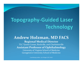
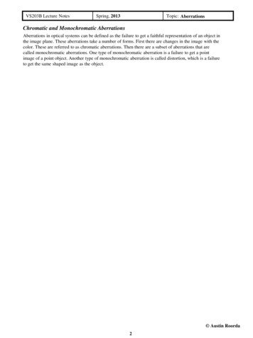
28JAMES C. WYANT AND KATHERINE CREATHVI. ZERNIKE POLYNOMIALSOften, to aid in the interpretation of optical test results it is convenient toexpress wavefront data in polynomial form. Zernike polynomials are oftenSagittalFocalSurfacePetzval SurfaceTangentialFocalSurfaceFIG. 33. Focal surfaces in presence of field curvature and astigmatism.

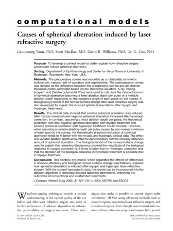
1. BASIC WAVEFRONT ABERRATION THEORYBarrel Distortion29Pincushion DistortionFIG. 34. Distortion,used for this purpose since they are made up of terms that are of the sameform as the types of aberrations often observed in optical tests (Zernike,1934). This is not to say that Zernike polynomials are the best polynomialsfor fitting test data. Sometimes Zernike polynomials give a terrible representation of the wavefront data. For example, Zernikes have little value when airturbulence is present. Likewise, fabrication errors present in the single-pointdiamond turning process cannot be represented using a reasonable numberof terms in the Zernike polynomial. In the testing of conical optical elements,additional terms must be added to Zernike polynomials to accuratelyrepresent alignment errors. Thus, the reader should be warned that the blinduse of Zernike polynomials to represent test results can lead to disastrousresults.Zernike polynomials have several interesting properties. First, they areone of an infinite number of complete sets of polynomials in two realvariables, ρ and θ′that are orthogonal in a continuous fashion over theinterior of a unit circle. It is important to note that the Zernikes areorthogonal only in a continuous fashion over the interior of a unit circle, andin general they will not be orthogonal over a discrete set of data points withina unit circle.Zernike polynomials have three properties that distinguish them fromother sets of orthogonal polynomials. First, they have simple rotationalsymmetry properties that lead to a polynomial product of the form(49)where G (θ′) is a continuous function that repeats itself every 2 π radians andsatisfies the requirement that rotating the coordinate system by an angle αdoes not change the form of the polynomial. That is,(50)

30JAMES C. WYANT AND KATHERINE CREATHThe set of trigonometric functions(51)where m is any positive integer or zero, meets these requirements.The second property of Zernike polynomials is that the radial functionmust be a polynomial in ρ of degree n and contain no power of ρ less than m.The third property is that R(p) must be even if m is even, and odd if m is odd.The radial polynomials can be derived as a special case of Jacobipolynomials, and tabulated asTheir orthogonality and normalizationproperties are given by(52)and(53)It is convenient to factor the radial polynomial into(54)whereasis a polynomial of order 2(n - m).can be written generally(55)In practice, the radial polynomials are combined with sines and cosinesrather than with a complex exponential. The final Zernike polynomial seriesfor the wavefront OPD W can be written as(56)whereis the mean wavefront OPD, and An, Bnm, and Cnm are individualpolynomial coefficients. For a symmetrical optical system, the wave aberrations are symmetrical about the tangential plane and only even functions of θ′are allowed. In general, however, the wavefront is not symmetric, and bothsets of trigonometric terms are included.Table III gives a list of 36 Zernike polynomials, plus the constant term.(Note that the ordering of the polynomials in the list is not universallyaccepted, and different organizations may use a different ordering.) Figures 35through 39 show contour maps of the 36 terms. Term #0 is a constant orpiston term, while terms # 1 and # 2 are tilt terms. Term # 3 represents focus.Thus, terms # 1 through # 3 represent the Gaussian or paraxial properties of

1. BASIC WAVEFRONT ABERRATION THEORY31

FIRST-ORDERn 1PROPERTIESn 2THIRD-ORDER ABERRATIONSASTIGMATISM AND DEFOCUSTILTCOMA AND TILTFOCUSTHIRD-ORDER SPHERICAL AND DEFOCUSF IG. 35. Two- and three-dimensional plots of Zernike poly-nomials # 1 to # 3.FIG. 36. Two- and three-dimensional plots of Zernike polynomials #4 to # 8.

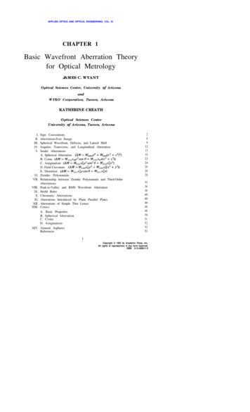
FIFTH-ORDERABERRATIONSFIG. 37. Two- and three-dimensional plots of Zernike polynomials # 9 to # 15.ABERRATIONSFIG. 38. Two- and three-dimensional plots of Zernike polynomials # 16 to # 24.

34JAMES C. WYANT AND KATHERINE CREATHn 5,6NINTH- & ELEVENTH-ORDER ABERRATIONSFIG. 39. Two- and three-dimensional plots of Zernike polynomials # 25 to # 36.the wavefront. Terms # 4 and # 5 are astigmatism plus defocus. Terms # 6and #7 represent coma and tilt, while term #8 represents third-orderspherical and focus. Likewise, terms # 9 through # 15 represent fifth-orderaberration, # 16 through # 24 represent seventh-order aberrations, and # 25through # 35 represent ninth-order aberrations. Each term contains theappropriate amount of each lower order term to make it orthogonal to eachlower order term. Also, each term of the Zernikes minimizes the rmswavefront error to the order of that term. Adding other aberrations of lowerorder can only increase the rms error. Furthermore, the average value of eachterm over the unit circle is zero.

1. BASIC WAVEFRONT ABERRATION THEORY35VII. RELATIONSHIP BETWEEN ZERNIKE POLYNOMIALS ANDTHIRD-ORDER ABERRATIONSFirst-order wavefront properties and third-order wavefront aberrationcoefficients can be obtained from the Zernike polynomials coefficients. Usingthe first nine Zernike terms Z0 to Z8, shown in Table III, the wavefront canbe written as(57)The aberrations and properties corresponding to these Zernike terms areshown in Table IV. Writing the wavefront expansion in terms of fieldindependent wavefront aberration coefficients, we obtain(58)Because there is no field dependence in these terms, they are not true Seidelaberrations. Wavefront measurement using an interferometer only providesdata at a single field point. This causes field curvature to look like focus, anddistortion to look like tilt. Therefore, a number of field points must bemeasured to determine the Seidel aberrations.Rewriting the Zernike expansion of Eq. (57), first- and third-order fieldindependent wavefront aberration terms are obtained. This is done byTABLE IVABERRATIONS CORRESPONDING TO THE FIRST NINE ZERNIKETERMSpistonx-tilty-tiltfocusastigmatism @ 0o & focusastigmatism @ 45o & focuscoma & x-tiltcoma & y-tiltspherical & focus

36JAMES C. WYANT AND KATHERINE CREATHgrouping like terms, and equating them with the wavefront aberrationcoefficients:pistontiltfocus astigmatismcomaspherical(59)Equation (59) can be rearranged using the identity(60)yielding terms corresponding to field-independent wavefront omaspherical(61)The magnitude, sign, and angle of these field-independent aberration termsare listed in Table V. Note that focus has the sign chosen to minimize themagnitude of the coefficient, and astigmatism uses the sign opposite thatchosen for focus.VIII. PEAK-TO-VALLEY AND RMS WAVEFRONT ABERRATIONIf the wavefront aberration can be described in terms of third-orderaberrations, it is convenient to specify the wavefront aberration by stating thenumber of waves of each of the third-order aberrations present. This method

371. BASIC WAVEFRONT ABERRATION THEORYTHIRD-ORDER ABERRATIONSTermDescriptionTABLE VIN TERMSOFZERNIKE COEFFICIENTSAngleMagnitudetiltfocussign chosen to minimize absolute valueof magnitudeastigmatismsign opposite that chosen in focus termcomasphericalNote: For angle calculations, if denominator 0, then angleangle 180o.for specifying a wavefront is of particular convenience if only a single thirdorder aberration is present. For more complicated wavefront aberrations it isconvenient to state the peak-to-valley (P-V) sometimes called peak-to-peak(P-P) wavefront aberration. This is simply the maximum departure of theactual wavefront from the desired wavefront in both positive and negativedirections. For example, if the maximum departure in the positive direction is 0.2 waves and the maximum departure in the negative direction is -0.1waves, then the P-V wavefront error is 0.3 waves.While using P-V to specify wavefront error is convenient and simple, itcan be misleading. Stating P-V is simply stating the maximum wavefronterror, and it is telling nothing about the area over which this error isoccurring. An optical system having a large P-V error may actually performbetter than a system having a small P-V error. It is generally moremeaningful to specify wavefront quality using the rms wavefront error.Equation (62) defines the rms wavefront error σ for a circular pupil, aswell as the variance σ2. W (ρ, θ) is measured relative to the best fit sphericalwave, and it generally has the units of waves. W is the mean wavefrontOPD.If the wavefront aberration can be expressed in terms of Zernike polynomials,

JAMES C. WYANT AND KATHERINE CREATH38the wavefront variance can be calculated in a simple form by using theorthogonality relations of the Zernike polynomials. The final result for theentire unit circle is(63)Table VI gives the relationship between σ and mean wavefront aberration forthe third-order aberrations of a circular pupil. While Eq. (62) could be used tocalculate the values of σ given in Table VI, it is easier to use linearcombinations of the Zernike polynomials to express the third-order aberrations, and then use Eq. (63).IX. STREHL RATIOWhile in the absence of aberrations, the intensity is a maximum at theGaussian image point. If aberrations are present this will in general no longerbe the case. The point of maximum intensity is called diffraction focus, and forsmall aberrations is obtained by finding the appropriate amount of tilt anddefocus to be added to the wavefront so that the wavefront variance is aminimum.The ratio of the intensity at the Gaussian image point (the origin of thereference sphere is the point of maximum intensity in the observation plane)in the presence of aberration, divided by the intensity that would be obtainedif no aberration were present, is called the Strehl ratio, the Strehl definition,or the Strehl intensity. The Strehl ratio is given by(64)TABLE VIRELATIONSHIPS BETWEEN WAVEFRONT ABERRATION MEAN ANDFIELD-INDEPENDENT THIRD-ORDER ABERRATIONSAberrationDefocusSphericalSpherical & DefocusAstigmatismAstigmatism & DefocusComaComa & Tilt WRMS FORσ