Transcription
Fast Fourier Transform andMATLAB ImplementationbyWanjun HuangforDr. Duncan L. MacFarlane1
SignalsIn the fields of communications, signal processing, and in electrical engineeringmore generally, a signal is any time‐varying or spatial‐varying quantityThis variable(quantity) changes in time Speech or audio signal: A sound amplitude that varies in time Temperature readings at different hours of a day Stock price changes over days Etc.EtcSignals can be classified by continues‐time signal and discrete‐time signal: A discrete signal or discrete‐time signal is a time series, perhaps a signal thath bhasbeen sampledl d ffrom a continuous‐timetitisignali l A digital signal is a discrete‐time signal that takes on only a discrete set ofvaluesDiscrete Time Signal10.50.5f[n]f(t)Continuous Time Signal10-0.5-10-0.501020Time (sec)3040-101020n30402
Periodic Signalperiodic signal and non‐periodic signal:Periodic SignalNon-Periodic Signal0-1 1f[n]f(t)101020Time (sec)30400-101020n3040Period T: The minimum interval on whicha signal repeatsFundamental frequency: f0 1/T1/THarmonic frequencies: kf0Any periodic signal can be approximatedbyy a sum of manyy sinusoids at harmonic frequenciesqof the signal(kfg ( f0) withappropriate amplitude and phaseInstead of using sinusoid signals, mathematically, we can use the complexexponential functions with both positive and negative harmonic frequenciesEuler formula: exp( j t ) sin( t ) j cos( t )3
Time‐Frequency Analysis A signal has one or more frequencies in it, and can be viewed fromtwo different standpoints: Time domain and Frequency domainTime Domian (Banded Wren Song)Frequency Domain2PowerAmplitudeA10-10246Sample Number8104x 100200400 600 800Frequency (Hz)1000 1200Time‐domain figure:ghow a signalg changesg over timeFrequency‐domain figure: how much of the signal lies within each givenfrequency band over a range of frequenciesWhy frequency domain analysis? To decompose a complex signal into simpler parts to facilitate analysis Differential and difference equations and convolution operations in thetime domain become algebraic operations in the frequency domain Fast Algorithm (FFT)4
Fourier TransformWe can go between the time domain and the frequency domainbyy usingg a tool called Fourier transformf A Fourier transform converts a signal in the time domain to thefrequency domain(spectrum) AnA iinverse FourierF i transformfconverts theh frequencyfdomaindicomponents back into the original time domain signalContinuous‐TimeContinuousTime Fourier Transform: F ( j ) f (t )e j tdt 1f (t ) 2 F ( j )ej td Discrete‐TimeDiscreteTime Fourier Transform(DTFT):X (ej ) x [ n ]en j nx[ n ] 12 X (e2 j )ej nd 5
Fourier Representation For Four Types of SignalsThe signal with different time‐domain characteristics has ntinues‐time periodic signal ‐‐‐ discrete non‐periodicspectrumpContinues‐time non‐periodic signal ‐‐‐ continues non‐periodicspectrumDiscrete nonnon‐periodicperiodic signal ‐‐‐ continues periodic spectrumDiscrete periodic signal ‐‐‐ discrete periodic spectrumThe last transformation between time‐domain and frequencyqy is mostusefulThe reason that discrete is associated with both time‐domain and frequencypcan onlyy take finite discrete time signalsgdomain is because computers6
Periodic SequenceA periodic sequence with period N is defined as: x (n) x ( n kN ), where k is integergFor example:Properties:W Nkn e j2 knNPeriodicSymmetricOrthogonal(it is called Twiddle Factor)W Nkn W N( k N ) n W Nk ( n N )W N kn (W Nkn ) * W N( N k ) n W Nk ( N n ) Nkn WN k 0 0N 1n rNotherFor a periodic sequence x (n) with period N, only N samplesare independent. So that N sample in one period is enough torepresent the whole sequence7
Discrete Fourier Series(DFS)Periodic signals may be expanded into a series of sine andcosine functionsN 1 X (k ) x ( n )W Nkn X ( k ) DFS ( x ( n )) x ( n ) IDFS ( X ( k ))n 01 N 1 kn x (n) X ( k )W NN n 0 X (k )is still a periodic sequence with period N in frequencydomainThe Fourier series for the discrete‐time periodic wave shown below:Sequence x (in time domain)Fourier 040102030408
Finite Length SequenceReal lift signal is generally afi i lengthfinitelh sequence x(n)x(n) 0If we periodic extend it by the period N,N then0 n N 1others x ( n ) x ( n rN )r x(n) x(n) 9
Relationship Between Finite Length Sequenceandd PeriodicP i di SequenceSA periodic sequence is the periodic extension of a finite lengthsequence x (n) x ( n rN ) x (( n ))m NA finite length sequence is the principal value interval of the periodicsequence0 n N 1 1x ( n) x ( n) R N ( n)Where R N (n ) 0So that:others x(n) x ( n ) R N ( n ) IDFS [ X ( k )] R N ( n ) X ( k ) X ( k ) R N ( k ) DFS [ x ( n )] R N ( n )10
Discrete Fourier Transform(DFT) Using the Fourier series representation we have DiscreteFourier Transform(DFT) for finite length signal DFT can convert time‐domain discrete signal into frequency‐domain discrete spectrumAssume that we have a signal { x [ n ]} nN 01 . Then the DFT of thesignal is a sequence X [ k ] for k 0 , , N 1N 1X [ k ] x [ n ] e 2 jnk/Nn 0The Inverse Discrete Fourier Transform(IDFT):1 N 12 jnkx[ n ] X [ k ]eN k 0/N, n 0 ,2 , , N 1 .Note that because MATLAB cannot use a zero or negativeindices, the index starts from 1 in MATLAB11
DFT ExampleThe DFT is widely used in the fields of spectral analysis,acoustics medical imaging,acoustics,imaging and telecommunications.telecommunicationsTime domain signal6For example:5x [ n ] [ 2 4 1 6 ], N 4 , ( n 0 ,1, 2 , 3 )3X [ k ] x [ n ]en 0 j 2nkAmplitudee43213 x [ n ] ( j ) nk0n 0-100.5X [ 0 ] 2 4 ( 1 ) 6 111.5Time22.532.53Frequency domain signal12108 X[k] X [1 ] 2 ( 4 j ) 1 6 j 3 2 jX [ 2 ] 2 ( 4 ) ( 1) 6 9X [3] 2 ( 4 j ) 1 6 j 3 2 j1642000.511.5Frequency212
Fast Fourier Transform(FFT) The Fast Fourier Transform does not refer to a new or differenttypeyp of Fourier transform. It refers to a veryy efficient algorithmgforcomputing the DFT The time taken to evaluate a DFT on a computer dependsprincipally on the number of multiplications involved. DFT needsN2 multiplications. FFT only needs Nlog2(N) The central insight which leads to this algorithm is therealization that a discrete Fourier transform of a sequence of Npoints can be written in terms of two discrete Fourier transformsof length N/2 Thus if N is a power of two,two it is possible to recursively applythis decomposition until we are left with discrete Fouriertransforms of single points13
Fast Fourier Transform(cont.)Re‐writingN 1X [ k ] x [ n ] e 2 jnk/Nn 0N 1X [ k ] x [ n ]W Nnkasn 0nkNIt is easy to realize that the same values of W are calculated many times as thecomputation proceedsUsing the symmetric property of the twiddle factor, we can save lots of computationsN 1X [ k ] x [ n ]Wn 0 N 2 1 x ( 2 r )W x 1 ( r )Wr 0N 2 1r 02 krN nkNN 1 x ( n )Wn 0even nN 2 1 knNN 1 x ( n )W Nknn 0odd nx ( 2 r 1 )W Nk ( 2 r 1 )r 0N 2 1krkW N 2Nr 0x 2 ( r )W Nkr 2 X 1 ( k ) W Nk X 2 ( k )Thus the N‐point DFT can be obtained from two N/2‐point transforms, one on eveninput data, and one on odd input data.14
Introduction for MATLABMATLAB is a numerical computing environment developed byMathWorks. MATLAB allows matrix manipulations,p, pplottingg offunctions and data, and implementation of algorithmsGetting helpYou can get help by typing the commands help or lookfor atthe prompt, e.g. help fftArithmetic operatorsSymbol Operation Example Addition31 93.1‐Subtraction 6.2 – 5* Multiplication 2 * 3/Division5/2 Power3 215
Data Representations in MATLABVariables: Variables are defined as the assignment operator “ ” . The syntax ofvariable assignment isvariablei bl name a valuel((oran expression)i )For example, x 5x 5 y [3*7, pi/3];% pi isin MATLAB Vectors/Matrices: MATLAB can create and manipulateVectors/Matricesmanip late arraysarra s of 1 (vectors),( ectors) 2(matrices), or more dimensionsrow vectors: a [1, 2, 3, 4] is a 1X4 matrixcolumn vectors: b [5; 6; 7; 8; 9] is a 5X1 matrix, e.g. A [1 2 3; 7 8 9; 4 5 6]A 1 2 37 8 94 5 616
Mathematical Functions in MATLABMATLAB offers many predefined mathematical functions fortechnical computing,pg, lSquare rootabs(x)angle(x)conj(x)log(x)Absolute valuePhase angleComplex conjugateNatural logarithmColon operator (:)Suppose we want to enter a vector x consisting of points(0,0.1,0.2,0.3, ,5). We can use the command x 0:0.1:5;;Most of the work you will do in MATLAB will be stored in files calledscripts, or m‐files, containing sequences of MATLAB commands to beexecuted over and over again17
Basic plotting in MATLABMATLAB has an excellent set of graphic tools. Plotting a given data set orthe results of computation is possible with very few commandsThe MATLAB command to plot a graph is plot(x,y), e.g.Sine function1 x 0:pi/100:2*pi;p /p ; y sin(x); plot(x,y)0.80.60.4MATLAB enables you to add axisLabels and titles, e.g.Sine of x0.20-0.2-0.4 xlabel('x 0:2\pi');\ i ylabel('Sine of x'); tile('Sine function')-0.6-0.8-10123456x 0:2x0:2 187
Example 1: Sine WaveSine Wave Signal1Amplitude0.50-0.5-100.20.40.60.81Time (s)Power Spectrum of a Sine Wave80PPower604020001020304050Frequency (Hz)607080Fs 150; % Sampling frequencyt 0:1/Fs:1; % Time vector of 1 secondf 5; % Create a sine wave of f Hz.x sin(2*pi*t*f);i (2* i*t*f)nfft 1024; % Length of FFT% Take fft, padding with zeros so that length(X)is equal to nfftX fft(x,nfft);% FFT is symmetric, throw away second halfX X(1:nfft/2);% Take the magnitude of fft of xmx abs(X);% Frequency vectorf (0:nfft/2-1)*Fs/nfft;% Generate the plot, title and labels.figure(1);plot(t,x);title('Sine Wave Signal');xlabel('Time (s)');ylabel('Amplitude');l b l('A lit d ')figure(2);plot(f,mx);title('Power Spectrum of a Sine Wave');xlabel('Frequency (Hz)');ylabel('Power');ylabel(Power );19
Example 2: Cosine WaveCosine Wave Signal1Amplitude0.50-0.5-100.20.40.60.81Time (s)Power Spectrum of a Cosine Wave80PPower604020001020304050Frequency (Hz)607080Fs 150; % Sampling frequencyt 0:1/Fs:1; % Time vector of 1 secondf 5; % Create a sine wave of f Hz.x cos(2*pi*t*f);nfft 1024; % Length of FFT% Take fft, padding with zeros so that length(X) isequal to nfftX fft(x,nfft);% FFT is symmetric,y, throw awayy second halfX X(1:nfft/2);% Take the magnitude of fft of xmx abs(X);% Frequency vectorf (0:nfft/2-1)*Fs/nfft;% Generate the plot, title and labels.figure(1);plot(t,x);title('Sine Wave Signal');xlabel('Time (s)');ylabel('Amplitude');ylabel(Amplitude );figure(2);plot(f,mx);title('Power Spectrum of a Sine Wave');xlabel('Frequency (Hz)');ylabel('Power');y20
Example 3: Cosine Wave with Phase ShiftCosine Wave Signal with Phase Shift1Amplitude0.50-0.5-100.20.40.60.81Time (s)Power Spectrum of a Cosine Wave Signal with Phase Shift80PPower604020001020304050Frequency (Hz)607080Fs 150; % Sampling frequencyt 0:1/Fs:1; % Time vector of 1 secondf 5; % Create a sine wave of f Hz.pha 1/3*pi; % phase shiftx cos(2*pi*t*f pha);nfft 1024; % Length of FFT% Take fft, padding with zeros so that length(X) isequal to nfftX fft(x,nfft);( ,)% FFT is symmetric, throw away second halfX X(1:nfft/2);% Take the magnitude of fft of xmx abs(X);% Frequency vectorf (0:nfft/2-1)*Fs/nfft;//% Generate the plot, title and labels.figure(1);plot(t,x);title('Sine Wave Signal');xlabel('Timexlabel(Time );title('Power Spectrum of a Sine Wave');qy (Hz)');xlabel('Frequencyylabel('Power');21
Example 4: Square WaveSquare Wave Signal1Amplitude0.50-0.5-100.20.40.6Time (s)0.81Power Spectrum of a Square Wave100Power80604020002040Frequency (Hz)6080Fs 150; % Sampling frequencyt 0:1/Fs:1; % Time vector of 1 secondf 5; % Create a sine wave of f Hz.x square(2*pi*t*f);nfft 1024; % Length of FFT% Take fft, padding with zeros so that length(X) isequal to nfftX fft(x,nfft);% FFT is symmetric,y, throw awayy second halfX X(1:nfft/2);% Take the magnitude of fft of xmx abs(X);% Frequency vectorf (0:nfft/2-1)*Fs/nfft;% Generate the plot, title and labels.figure(1);plot(t,x);title('Square Wave Signal');xlabel('Time (s)');ylabel('Amplitude');ylabel(Amplitude );figure(2);plot(f,mx);title('Power Spectrum of a Square Wave');xlabel('Frequency (Hz)');yylabel('Power');22
Example 5: Square PulseSquare Pulse Signal1Amplitude0.80.60.40.20-0.50Time (s)0.5Power Spectrum of a Square Pulse3025Power2015105002040Frequency (Hz)6080Fs 150; % Sampling frequencyt -0.5:1/Fs:0.5; % Time vector of 1 secondw .2; % width of rectanglex rectpuls(t,rectpuls(t w); % Generate Square Pulsenfft 512; % Length of FFT% Take fft, padding with zeros so that length(X) isequal to nfftX fft(x,nfft);% FFT is symmetric,y, throw awayy second halfX X(1:nfft/2);% Take the magnitude of fft of xmx abs(X);% Frequency vectorf (0:nfft/2-1)*Fs/nfft;% Generate the plot, title and labels.figure(1);plot(t,x);title('Square Pulse Signal');xlabel('Time (s)');ylabel('Amplitude');ylabel(Amplitude );figure(2);plot(f,mx);title('Power Spectrum of a Square Pulse');xlabel('Frequency (Hz)');yylabel('Power');23
Example 6: Gaussian PulseGaussian Pulse Signal4Amplitude3210-0.50Time (s)0.5Power Spectrum of a Gaussian Pulse6050Powerr40302010005101520Frequency (Hz)25Fs 60; % Sampling frequencyt -.5:1/Fs:.5;x 1/(sqrt(2*pi*0.01))*(exp(-t. 2/(2*0.01)));nfft 1024; % Length of FFT% Take fft, padding with zeros so thatlength(X) is equal to nfftX fft(x,nfft);% FFT is symmetric, throw away second halfX X(1:nfft/2);()% Take the magnitude of fft of xmx abs(X);% This is an evenly spaced frequency vectorf (0:nfft/2-1)*Fs/nfft;% Generate the plot, title and labels.figure(1);plot(t,x);title('Gaussian Pulse Signal');xlabel('Time le('Power Spectrum of a Gaussian Pulse');xlabel('Frequency (Hz)');ylabel('Power');3024
Example 7: Exponential DecayExponential Decay Signal2Amplitude1.510.5000.20.40.6Time (s)0.81PPowerSSpectrumtoff ExponentialEti l DecayDSiSignall7060Poweer5040302010002040Frequency (Hz)6080Fs 150; % Sampling frequencyt 0:1/Fs:1; % Time vector of 1 secondx 2*exp(-5*t);nfft 1024;1024 % Length of FFT% Take fft, padding with zeros so thatlength(X) is equal to nfftX fft(x,nfft);% FFT is symmetric, throw away secondhalfX X(1:nfft/2);% Take the magnitude of fft of xmx abs(X);% This is an evenly spaced frequencyvectorf (0:nfft/2-1)*Fs/nfft;% Generate the plot, title and labels.figure(1);plot(t,x);title('Exponential Decay Signal');xlabel('Time le('Power Spectrum of Exponentialy Signal');g);Decayxlabel('Frequency (Hz)');ylabel('Power');25
Example 8: Chirp SignalChirp Signal1Amplitude0.50-0.5-100.20.40.6Time (s)0.81Power Spectrumpof Chirpp Signalg25Powwer201510500204060Frequency (Hz)80100Fs 200; % Sampling frequencyt 0:1/Fs:1; % Time vector of 1 secondx chirp(t,0,1,Fs/6);nfft 1024;; % Lengthgof FFT% Take fft, padding with zeros so thatlength(X) is equal to nfftX fft(x,nfft);% FFT is symmetric, throw away second halfX X(1:nfft/2);% Take the magnitude of fft of xmx abs(X);% This is an evenly spaced frequencyvectorf (0:nfft/2-1)*Fs/nfft;% Generate the plotplot, title and labelslabels.figure(1);plot(t,x);title('Chirp Signal');xlabel('Time itle('Power Spectrum of Chirp Signal');xlabel('Frequency (Hz)');ylabel('Power');26
Periodic Signal periodic signal and non‐periodic signal: 1 Periodic Signal 1 Non-Period