Transcription
Exponential smoothing:The state of the art – Part IIEverette S. Gardner, Jr.Bauer College of Business334 Melcher HallUniversity of HoustonHouston, Texas 77204-6021Telephone 713-743-4744, Fax 713-743-4940egardner@uh.eduJune 3, 2005
Exponential smoothing: The state of the art – Part II
Exponential smoothing: The state of the art – Part IIAbstractIn Gardner (1985), I reviewed the research in exponential smoothing since the originalwork by Brown and Holt. This paper brings the state of the art up to date. The most importanttheoretical advance is the invention of a complete statistical rationale for exponential smoothingbased on a new class of state-space models with a single source of error. The most importantpractical advance is the development of a robust method for smoothing damped multiplicativetrends. We also have a new adaptive method for simple smoothing, the first such method todemonstrate credible improved forecast accuracy over fixed-parameter smoothing.Longstanding confusion in the literature about whether and how to renormalize seasonal indicesin the Holt-Winters methods has finally been resolved. There has been significant work inforecasting for inventory control, including the development of new prediction distributions fortotal lead-time demand and several improved versions of Croston’s method for forecastingintermittent time series. Regrettably, there has been little progress in the identification andselection of exponential smoothing methods. The research in this area is best described asinconclusive, and it is still difficult to beat the application of a damped trend to every time series.Key wordsTime series – ARIMA, exponential smoothing, state-space models, identification, stability,invertibility, model selection; Comparative methods – evaluation; Intermittent demand;Inventory control; Prediction intervals; Regression – discount weighted, kernel
1. IntroductionWhen Gardner (1985) appeared, many believed that exponential smoothing should bedisregarded because it was either a special case of ARIMA modeling or an ad hoc procedurewith no statistical rationale. As McKenzie (1985) observed, this opinion was expressed innumerous references to my paper. Since 1985, the special case argument has been turned on itshead, and today we know that exponential smoothing methods are optimal for a very generalclass of state-space models that is in fact broader than the ARIMA class.This paper brings the state of the art in exponential smoothing up to date with a criticalreview of the research since 1985. Prior research findings are included where necessary toprovide continuity and context. The plan of the paper is as follows. Section 2 summarizes newinformation that has come to light on the early history of exponential smoothing. Section 3 givesformulations for the standard Holt-Winters methods and a number of variations and extensions tocreate equivalences to state-space models, normalize seasonals, and cope with problems such asseries with a fixed drift, missing observations, irregular updates, planned discontinuities,multiple seasonal cycles (in the same series), and multivariate series. Equivalent regression,ARIMA, and state-space models are reviewed in Section 4. This section also discussesvariances, prediction intervals, and some possible explanations for the robustness of exponentialsmoothing. Procedures for method and model selection are discussed in Section 5, including theuse of time series characteristics, expert systems, information criteria, and operational measures.Section 6 reviews the details of model-fitting, including the selection of parameters, initialvalues, and loss functions. In Section 6, we also discuss the use of adaptive parameters to avoidmodel-fitting. Applications of exponential smoothing to inventory control with both continuousand intermittent demand are discussed in Section 7. Section 8 summarizes the many empirical1
studies in which exponential smoothing has been used. Conclusions and an assessment of thestate of the art are offered in Section 9. This plan does not include coverage of tracking signals,a subject that has disappeared from the literature since the earlier paper.2. Early history of exponential smoothingExponential smoothing originated in Robert G. Brown’s work as an OR analyst for theUS Navy during World War II (Gass and Harris, 2000). In 1944, Brown was assigned to theantisubmarine effort and given the job of developing a tracking model for fire-controlinformation on the location of submarines. This information was used in a mechanicalcomputing device, a ball-disk integrator, to estimate target velocity and the lead angle for firingdepth charges from destroyers. Brown’s tracking model was essentially simple exponentialsmoothing of continuous data, an idea still used in modern fire-control equipment.During the early 1950s, Brown extended simple exponential smoothing to discrete dataand developed methods for trends and seasonality. One of his early applications was inforecasting the demand for spare parts in Navy inventory systems. The savings in data storageover moving averages led to the adoption of exponential smoothing throughout Navy inventorysystems during the 1950s. In 1956, Brown presented his work on exponential smoothing ofinventory demands at a conference of the Operations Research Society of America. Thispresentation formed the basis of Brown’s first book, Statistical Forecasting for InventoryControl (Brown, 1959). His second book, Smoothing, Forecasting, and Prediction of DiscreteTime Series (Brown, 1963), developed the general exponential smoothing methodology. Innumerous later books, Brown integrated exponential smoothing with inventory management andproduction planning and control.2
During the 1950s, Charles C. Holt, with support from the Logistics Branch of the Officeof Naval Research (ONR), worked independently of Brown to develop a similar method forexponential smoothing of additive trends and an entirely different method for smoothingseasonal data. Holt’s original work was documented in an ONR memorandum (Holt, 1957) andwent unpublished until recently (Holt, 2004a, 2004b). However, Holt’s ideas gained widepublicity in 1960. In a landmark article, Winters (1960) tested Holt’s methods with empiricaldata, and they became known as the Holt-Winters forecasting system. Another landmark articleby Muth (1960) was among the first to examine the optimal properties of exponential smoothingforecasts. Holt’s methods of exponential smoothing were also featured in the classic text byHolt, Modigliani, Muth, and Simon, Planning Production, Inventories, and Work Force (1960),a book that is still in use today in doctoral programs in operations management.3. Formulation of exponential smoothing methodsSection 3.1 classifies and gives formulations for the standard methods of exponentialsmoothing. These methods can be modified to create state-space models as discussed in Section3.2. Seasonal indices are not automatically renormalized in either the standard or state-spaceversions of exponential smoothing, and procedures for renormalization are reviewed in Section3.3. In Section 3.4, we collect a number of variations on the standard methods to cope withspecial kinds of time series.3
3.1 Standard methodsTable 1 contains equations for the standard methods of exponential smoothing, all ofwhich are extensions of the work of Brown (1959, 1963), Holt (1957), and Winters (1960). Foreach type of trend, and for each type of seasonality, there are two sections of equations. The firstsection gives recurrence forms and the second gives error-correction forms. Recurrence formswere used in the original work by Brown and Holt and are still widely used in practice, but errorcorrection forms are simpler and give equivalent forecasts. The notation follows Gardner (1985)and is defined in Table 2. It is worth emphasizing that there is still no agreement on notation forexponential smoothing. An appalling variety of notation exists in the literature, and someauthors add to the confusion by changing notation from one paper to the next.Hyndman et al.’s (2002) taxonomy, as extended by Taylor (2003a), is helpful indescribing the methods. Each method is denoted by one or two letters for the trend (rowheading) and one letter for seasonality (column heading). Method N-N denotes no trend with noseasonality, or simple exponential smoothing (Brown, 1959). The other nonseasonal methodsare Holt’s (1957) additive trend (A-N), Gardner and McKenzie’s (1985) damped additive trend(DA-N), Pegels’ (1969) multiplicative trend (M-N), and Taylor’s (2003a) damped multiplicativetrend (DM-N). The parameters in the trend methods can be constrained using discounted leastsquares (DLS) to produce special cases often called Brown’s methods, as discussed in Section4.1. All seasonal methods are formulated by extending the methods in Winters (1960). Notethat the forecast equations for the seasonal methods are valid only for a forecast horizon ( m )less than or equal to the length of the seasonal cycle ( p ).4
Table 1Standard exponential smoothing methodsSeasonalityTrendNNoneS t αX t (1 α ) S t 1Xˆ ( m) SAAdditiveS t α ( X t I t p ) (1 α )S t 1MMultiplicativeS t α ( X t / I t p ) (1 α )S t 1I t δ ( X t S t ) (1 δ ) I t pXˆ t (m) S t I t p mI t δ ( X t / S t ) (1 δ ) I t pXˆ t (m) S t I t p mS t S t 1 αetXˆ t (m) S tS t S t 1 αetS t S t 1 αet / I t pI t I t p δ (1 α )etXˆ t (m) S t I t p mI t I t p δ (1 α )et / S tXˆ t (m) S t I t p mS t αX t (1 α )(S t 1 Tt 1 )S t α ( X t I t p ) (1 α )(S t 1 Tt 1 )S t α ( X t / I t p ) (1 α )(S t 1 Tt 1 )Tt γ ( S t S t 1 ) (1 γ )Tt 1Xˆ t (m) St mTtTt γ ( S t S t 1 ) (1 γ )Tt 1Tt γ ( S t S t 1 ) (1 γ )Tt 1I t δ ( X t S t ) (1 δ ) I t pXˆ t ( m ) S t mTt I t p mI t δ ( X t / S t ) (1 δ ) I t pXˆ t (m) ( St mTt ) I t p mSt St 1 Tt 1 αetSt St 1 Tt 1 αetS t S t 1 Tt 1 αet / I t pTt Tt 1 αγ e tXˆ t (m) St mTtTt Tt 1 αγ e tTt Tt 1 αγet / I t pS t αX t (1 α )(S t 1 φTt 1 )S t α ( X t I t p ) (1 α )(S t 1 φTt 1 )S t α ( X t / I t p ) (1 α )(S t 1 φTt 1 )Tt γ (S t S t 1 ) (1 γ )φTt 1Tt γ (S t S t 1 ) (1 γ )φTt 1Tt γ (S t S t 1 ) (1 γ )φTt 1I t δ ( X t S t ) (1 δ ) I t pI t δ ( X t / S t ) (1 δ ) I t ptNNoneAAdditivetmIt It p δ (1 α )etXˆ t ( m ) St mTt I t p mXˆ t ( m ) S t φ Ttii 1DADampedAdditivemmXˆ t ( m ) S t φ Ttii 1Xˆ t ( m ) ( S t φ i Tt ) I t p mS t S t 1 φTt 1 α e tTt φTt 1 αγ e tS t S t 1 φTt 1 α et / I t pIt It p δ (1 α )etTt φTt 1 αγ et / I t pI t I t p δ (1 α )et / StXˆ t ( m ) ( S t φ i Tt ) I t p mS t α X t (1 α )( S t 1 Rt 1 )S t α ( X t I t p ) (1 α ) S t 1 Rt 1S t α ( X t / I t p ) (1 α ) S t 1 Rt 1Rt γ (S t / S t 1 ) (1 γ ) Rt 1Xˆ t (m) St RtmRt γ (S t / S t 1 ) (1 γ ) Rt 1Rt γ (S t / S t 1 ) (1 γ ) Rt 1I t δ ( X t S t ) (1 δ ) I t pXˆ t ( m ) S t Rtm I t p mI t δ ( X t / S t ) (1 δ ) I t pXˆ t ( m ) ( S t Rtm ) I t p mS t S t 1 Rt 1 αetS t S t 1 Rt 1 αetS t S t 1 Rt 1 αet / I t pR t R t 1 αγ e t / S t 1Xˆ (m) S R mR t R t 1 αγ e t / S t 1I t I t p δ (1 α )etXˆ t ( m ) S t Rtm I t p mRt Rt 1 (αγet / S t 1 ) / I t pI t I t p δ (1 α )et / S tXˆ t (m) ( S t Rtm ) I t p mSt αX t (1 α )(St 1 Rtφ 1 )S t α ( X t I t p ) (1 α ) S t 1 Rtφ 1S t α ( X t I t p ) (1 α )( S t 1 Rtφ 1 )Rt γ ( S t / S t 1 ) (1 γ ) Rtφ 1I t δ ( X t S t ) (1 δ ) I t pRt γ ( S t S t 1 ) (1 γ ) Rtφ 1I t δ ( X t S t ) (1 δ ) I t 1 φXˆ t ( m) S t Rt i 1 I t p m φXˆ t ( m) ( S t Rt i 1 ) I t p mS t S t 1 Rtφ 1 αetS t S t 1 Rtφ 1 αet / I t pRt Rtφ 1 αγ et / S t 1I t I t p δ (1 α )etRt Rtφ 1 (αγet / S t 1 ) / I t ptttRt γ ( S t / S t 1 ) (1 γ ) Rtφ 1Xˆ t ( m) DMDampedMultiplicativei 1mXˆ t ( m ) S t φ i Tt I t p mi 1MMultiplicativemXˆ t ( m ) S t φ i Tt I t p mi 1S t S t 1 φTt 1 α e tTt φTt 1 αγ e tI t I t p δ (1 α )et / S tXˆ t (m) ( St mTt ) I t p mi m φS t Rt i 1St St 1Rtφ 1 αetR t R tφ 1 αγ e t / S t 1 φXˆ t ( m) S t Rt i 1mimXˆ t ( m) m φS t Rt i 1ii I t p mmi 1miI t I t p δ (1 α )et / S t φXˆ t ( m) ( S t Rt i 1 ) I t p mmi5
Table 2. Notation for exponential smoothingSymbolDefinitionαγδφβSmoothing parameter for the level of the seriesSmoothing parameter for the trendSmoothing parameter for seasonal indicesAutoregressive or damping parameterDiscount factor, 0 β 1StSmoothed level of the series, computed after X t is observed. Also the expected valueof the data at the end of period t in some modelsTtSmoothed additive trend at the end of period tRtSmoothed multiplicative trend at the end of period tItSmoothed seasonal index at the end of period t . Can be additive or multiplicativeXtObserved value of the time series in period tmNumber of periods in the forecast lead-timepNumber of periods in the seasonal cycleˆX t ( m ) Forecast for m periods ahead from origin tetOne-step-ahead forecast error, et X t Xˆ t 1 (1). Note that et ( m ) should be used forother forecast originsCtCumulative renormalization factor for seasonal indices. Can be additive ormultiplicativeVtTransition variable in smooth transition exponential smoothingDtObserved value of nonzero demand in the Croston methodQtObserved inter-arrival time of transactions in the Croston methodZtSmoothed nonzero demand in the Croston methodPtSmoothed inter-arrival time in the Croston methodYtEstimated demand per unit time in the Croston method ( Z t Pt )6
There are several differences between Table 1 and the tables of equations in Gardner(1985). First, the DA methods are given in recurrence forms that were not included in the earlierpaper. Second, the seasonal DA methods were formulated with three parameters in the earlierpaper, but the same methods in Table 1 contain four parameters as developed in Gardner andMcKenzie (1989). Finally, the DM methods are new.The DA-N method can be used to forecast multiplicative trends with the autoregressiveor damping parameter φ restricted to the range 1 φ 2 , a method sometimes called“generalized Holt.” As Taylor (2003a) observed, generalized Holt is a clumsy way to model amultiplicative trend because the local slope is estimated by smoothing successive differences ofthe local level. In contrast, Pegels’ multiplicative trends (M-N, M-A, and M-M) estimate thelocal growth rate by smoothing successive ratios of the local level. In hopes of producing morerobust forecasts, Taylor’s methods (DM-N, DM-A, and DM-M) add a damping parameterφ 1 to Pegels’ multiplicative trends.Although many new models underlying exponential smoothing have been proposed since1985, the damped multiplicative trends are the only new methods in the sense that they createnew forecast profiles. Like the damped additive trends, the forecast profiles for Taylor’smethods will eventually approach a horizontal nonseasonal or seasonally-adjusted asymptote.However, in the near term, different values of φ can be used to produce forecast profiles that areconvex, nearly linear, or even concave.7
3.2 State-space equivalent methodsThere are many equivalent state-space models for each of the methods in Table 1. Herewe review the particular modeling framework of Hyndman et al. (2002) that includes all methodsin Table 1 except the DM methods. In this framework, each exponential smoothing method hastwo corresponding state-space models, each with a single source of error (SSOE). One modelhas an additive error and the other has a multiplicative error. As discussed in Section 4.3, if theparameters are the same, the two models give the same point forecasts but different variances.The methods corresponding to the Hyndman et al. framework are the same as those in Table 1with two exceptions: we must modify all multiplicative seasonal methods and all dampedadditive-trend methods.We proceed as follows to modify the multiplicative seasonal methods. In the N-Mstandard equations for updating the multiplicative seasonal component I t , replace the smoothedlevel S t with S t 1 . This change is made in both recurrence and error-correction forms. In the AM, DA-M, and M-M standard equations for updating I t , replace S t with S t 1 Tt 1 , where Tt 1is the previous smoothed trend, again in both recurrence and error-correction forms. In the DAM method, note that the seasonal state-space modification does not damp Tt 1 in updating I t .Koehler et al. (2001) present several other state-space versions of the A-M method, allwith the same multiplicative seasonal modification. One precedent for this modification is foundin Williams (1987), who shows that it allows us to update each component independently, whilein the standard method the new smoothed level is used in updating the other components.Archibald (1990) made the same point without reference to the work of Williams. Perhapsanother reason to use the multiplicative seasonal modification is that, as Ord (2004) observed,8
this was done in Holt’s original work (1957). However, Holt et al. (1960) and Winters (1960)discarded this idea and used the standard equations in Table 1.What are the practical consequences of adopting the state-space versions of themultiplicative seasonal methods? The answer to this question awaits empirical study. In ananalysis of the A-M method, Koehler et al. (2001) show that the difference between the twoversions of the equation for updating the seasonal component will be small, provided that allthree smoothing parameters are less than about 0.3. However, Koehler et al. warn that negativeseasonal components can occur in the state-space version of A-M unless the forecast errors aremuch less variable than the data.To make the damped additive (DA) methods fit the Hyndman et al. (2002) framework,we begin with the level equations. The equivalent state-space model does not damp the previoustrend in the level equations, so we delete φ (replace φTt 1 with Tt 1 ). Next, the forecastequations must be changed to begin damping at two steps ahead, rather than immediately as inTable 1. The forecast equation in the nonseasonal state-space equivalent method (DA-N) is:m 1Xˆ t (m) ( S t φ i Tt )(1)i 0At first glance, it looks as if the state-space DA method will always extrapolate more trend at anyhorizon than the standard method, but this may not be true if fitted parameter values differsubstantially between the two versions. Given the success of the standard DA method, it isdifficult to understand why Hyndman et al. (2002) chose to start trend damping at two stepsahead. There appears to be no statistical reason for this choice. In contrast to Hyndman et al.,the text by Bowerman et al. (2005) includes a comprehensive treatment of state-space models forexponential smoothing in which trend damping starts immediately.9
3.3 Renormalization of seasonal indicesThe standard seasonal methods are initialized so that the average seasonal index is 0(additive) or 1 (multiplicative); thereafter, normalization goes astray because only one seasonalindex is updated each period. The problem of renormalization was overlooked in Gardner(1985) and there has been much confusion in the literature about whether it is necessary torenormalize the seasonal indices, and if so when and how this should be done.Lawton (1998) analyzed an equivalent state-space model for the A-A method and reachedseveral conclusions. First, if seasonal indices in the A-A method are not renormalized, estimatesof trend are correct although estimates of level and seasonals are biased. Fortunately, the errorsin estimating level and seasonals are counter-balancing and do not impact the forecasts. Ifrenormalization of seasonal indices alone is carried out, a very common procedure in practice,this must be done at every time period or the forecasts will be biased until the A-A equationshave sufficient time to adjust the level. Lawton gives an example in which the bias is seriouscompared to not renormalizing. If we choose to renormalize at an interval other than every timeperiod, the procedure is as follows: (1) subtract a constant value from each seasonal index toforce the sum to zero, and (2) add the same constant to the level.Other A-A renormalization equations are found in Roberts (1982), McKenzie (1986), andNewbold (1988). These authors go about renormalization in different ways, but their pointforecasts turn out to be the same. Furthermore, the point forecasts from all of the alternative setsof renormalization equations are the same as the point forecasts from the standard equations.McKenzie showed that the link between the standard and renormalized versions of the A-Amethod is very simple. The two methods give equivalent forecasts if we replace the levelparameter α in the standard error-correction form with (α δ p) , where δ is the smoothing10
parameter for the seasonal component and p is the number of periods in one season. Thisparameter adjustment should occur automatically during model-fitting.Prior to Archibald and Koehler (2003), the only renormalization equations for the A-Mmethod were those of Roberts (1982) and McKenzie (1986). Archibald and Koehler found thatthe Roberts and McKenzie equations result in point forecasts that differ from each other and alsofrom the standard-equation forecasts. Therefore, Archibald and Koehler set out to make sense ofthe renormalization problem. First, they developed new renormalization equations for the A-Mmethod that give the same point forecasts as the standard equations. Second, they developedanalogous A-A renormalization equations. Finally, they derived equations that computecumulative renormalization correction factors for the A-A and A-M methods. These correctionfactors should prove to be popular in practice because they allow the user to keep the standardequations and renormalize the seasonal indices at any point in time.The cumulative renormalization correction factor C t for the A-A method is computediteratively using a simple equation:C t C t 1 δ et p ,(2)To renormalize at any time, add C t to the level and subtract it from each seasonal index.Archibald and Koehler derived the cumulative renormalization correction factor for theA-M method using the state-space version. Here we give the correction factor for the standardA-M version in Table 1:C t C t 1 (1 δ et pS t )(3)To renormalize at any time, multiply level and trend by C t and divide each seasonal index byC t . If the state-space A-M version is used, replace S t with S t 1 Tt 1 in equation (3).11
To sum up the research in this area, there is no reason to renormalize in the additiveseasonal methods if forecast accuracy is the only concern. It is not known whetherrenormalization can safely be ignored in the multiplicative methods. If we choose to renormalizeto provide reliable estimates of either additive or multiplicative model components, the simplestapproach is to apply the correction factors of Archibald and Koehler. Their A-A and A-Mcorrection factors are easily extended to the other seasonal methods in either standard or statespace form.There is little empirical evidence on the problem of renormalization. The only referenceis Archibald and Koehler (2003), who tested the 401 monthly series from the M1-Competition(Makridakis et al., 1982). In 12 series, they found that the standard A-A method produced valuesof level, trend, and seasonal indices that were off more than 5% (compared to renormalized AA).3.4 Other variations on the standard methodsThis section collects special versions of the standard Holt-Winters methods to cope withmissing or irregular observations, irregular update intervals, planned discontinuities, seriescontaining a fixed drift, and series containing two or more seasonal cycles. We can also simplifythe A-A method by merging the level and seasonal components, and adapt several methods tomultivariate series. Discussion of one additional variation, Croston’s (1972) method forinventory series with intermittent demands, is deferred until Section 7 on inventory control.For missing observations, Wright’s (1986a, 1986b) solution is straightforward. Missingobservations receive zero weight, while the others are exponentially weighted according to theage of the observation. Wright gives modified formulas for the N-N and A-N methods thatautomatically adjust the weighting pattern for all observations following a gap. These formulas12
also work for the equivalent problem of observations that naturally occur at irregular timeintervals. Wright’s procedure was extended by Cipra et al. (1995) to seasonal methods.Although Wright’s procedure looks sensible, Aldrin and Damsleth (1989) made a complaint thathas been repeated many times in the literature of exponential smoothing, that the procedure is adhoc with no statistical rationale. Aldrin and Damsleth developed an elaborate alternativeprocedure that computes optimal weights in the equivalent ARIMA models. It is not clear thatthe ARIMA procedure is worth the trouble because the authors analyzed two time series and gotabout the same results as the Wright procedure.If the time between updates of the N-N method is irregular, the data for several periodsmay be reported as a combined observation. Obviously, the smoothing parameter should beincreased to give more weight to combined observations. Johnston (1993) derived a formula foroptimal adjustment of the smoothing parameter, while Anderson (1994) and Walton (1994)derived simpler alternative formulas. Anderson’s idea is the simpler of the two, and gives valuesvery close to Johnston’s optimal formula. When a combined observation occurs, in the N-Nequation we replace X t with X t / k , where k is the number of periods combined, and wereplace α with the expression 1 (1 α ) k . This adjustment assumes that the data are spreadevenly over the combined periods.There may be planned discontinuities in a time series. For example, we may expect adisruption in demand following a price change or a new product introduction. There are threeways of dealing with planned discontinuities in exponential smoothing. If discontinuities arerecurring, Carreno and Madinaveitia (1990) add an index similar to a seasonal index to the A-Nmethod to model the effects. When the effects of discontinuities cannot be estimated fromhistory, judgmental adjustments to the forecasts are usually necessary. Williams and Miller13
(1999) recommend making such adjustments within the exponential smoothing method ratherthan as a second-stage correction outside the method. The basic idea is to add an adjustmentfactor to the forecast equation and otherwise allow the updating equations to operate normally.If the discontinuity occurs approximately as planned, this will be more accurate than makingsecond-stage corrections outside the method. It may be possible to express planneddiscontinuities as a set of linear restrictions on the forecasts from a linear exponential smoothingmethod. If so, Rosas and Guerrero (1994) show that one can compute weights that meet therestrictions in the moving-average representation of the equivalent ARIMA model. Once this isdone, the weights can be converted into smoothing parameters.The N-N method can be enhanced by adding a drift (fixed trend) term, making themethod equivalent to the “Theta method of forecasting” (Assimakopoulos and Nikolopoulos,2000) that performed well in the M3 competition (Makridakis and Hibon, 2000). In amathematical tour de force, Hyndman and Billah (2003) showed that the Theta method is thesame thing as simple smoothing with drift equal to half the slope of a linear trend fitted to thedata. Another way to match the Theta method is to use the same drift choice in the A-N methodwith the trend parameter set to zero. We do not know why the particular drift choice in the Thetamethod or its equivalents is better than any other, nor is it clear when one should prefer a fixeddrift over a smoothed trend.For time series containing two seasonal cycles, Taylor (2003b) adds one more seasonalcomponent to the A-M method. The new method, called double seasonal exponential smoothing,was applied to electricity demand recorded at half-hour intervals, with one seasonal equation fora within-day seasonal cycle and another for a within-week cycle. As often happens in complextime series forecasted with exponential smoothing, Taylor found significant first-orderautocorrelation in the residuals. Thus he fitted an AR(1) model to remove it, estimating the14
AR(1) parameter at the same time as the smoothing parameters. The resulting forecastsoutperformed those from the standard A-M method as well as a double seasonal ARIMA model.Rather than add a seasonal component, Snyder and Shami (2001) eliminate it from the AA method. The seasonal component is incorporated into the level, which depends on the level ayear ago and is augmented by the total growth in all seasons during the past year. Thus theirparsimonious method requires only two parameters. Snyder and Shami found that the twoparameter version of A-A was less accurate than the standard three-parameter version, althoughthe differences were not statistically significant. Snyder and Shami overlooked a simpler way toreduce the number of parameters in any of the trend and seasonal methods, which is to applyDLS, as discussed in Section 4.1.Some of the
class of state-space models that is in fact broader than the ARIMA class. This paper brings the state of the art in exponential smoothing up to date with a critical review of the research since 1985. Prior research findings are included where necessary to provide con
