Transcription
2021, vol. 21, no. 1, PUTERCOMPUTERMETHODSIN MATERIALSSCIENCEMETHODSIN MATERIALSSCIENCEA numerical simulation study ofmold filling in the injection molding processCOMPUTER METHODS IN MATERIALS SCIENCEMarkus Baum*, Denis AndersCologne University of Applied Sciences (TH Köln), Group for Computational Mechanics and Fluid Dynamics, Steinmüllerallee 1, 51643 Gummersbach, Germany.AbstractInjection molding can undoubtedly be regarded as one of the most widely used manufacturing processes for polymers (Guevara-Morales & Figueroa-Lopez, 2014). Furthermore, injection molding has found its way into various branches of industry(Fernandez et al., 2018) since it has several essential advantages over other processing techniques in terms of good surfacefinish, the ability to process complex parts without the need for secondary operations, and low cost for mass production. Inorder to find optimal process settings, it is necessary to gain a deeper insight into the filling process and the underlying physicalphenomena, as well as a thorough understanding of the complex material behavior. In this context, the numerical simulation ofthe injection molding process is increasingly important. Therefore, the current contribution is dedicated to present a thoroughcomparative numerical study for the mold filling of an exemplary thin-walled mold geometry, including a realistic non-Newtonian viscosity model for the polymer melt. For the numerical simulation, the authors employ the commercial CFD softwarepackages Cadmould 3D-F and ANSYS CFX. While ANSYS CFX is a well-established CFD software for numerical modellingof multiphysical phenomena, Cadmould 3D-F is a highly specialized and computationally efficient alternative suitable forcertain geometric configurations in the context of injection molding. The present study is new in the sense that it demonstratesthe equivalence of the considered software packages for the simulation of the injection molding process in thin-walled moldgeometries.Keywords: injection molding, polymers, Hele-Shaw approximation, computational fluid dynamics, computing methodsefficiency and product quality. In the context of injectionmolding, mass homogeneity and high dimensional accuracy, minimization of shrinkage and warpage, surfacestructure (degree of gloss and the surface quality), andstrength properties (e.g., fiber orientation for glass fiber reinforced plastics) are typical indicators for product quality.Optimization of product quality, on the one hand,while minimizing process costs on the other requires anin-depth understanding of the injection molding process.In this context, injection molding simulation plays an essential role. The main objective is to determine the influence of adjustable process variables such as mold cavitycharacteristics, gating and temperature control system,1. IntroductionIn the course of globalization, injection molding (IM)has seen rapid technological development and openedup new fields of application for electronic componentsdevices, medical devices as well as in the automotive/transport industry and packaging industry. Alongsideextrusion, injection molding is one of the most important primary forming manufacturing processes in theplastics processing industry.The growing competition on the global market forplastic products results in increased demands on process* C orresponding author: markus.baum@th-koeln.deORCID ID’s: 0000-0001-5840-1374 (M. Baum), 0000-0002-7849-0666 (D. Anders) 2021 Authors. This is an open access publication, which can be used, distributed and reproduced in any medium according to theCreative Commons CC-BY 4.0 License requiring that the original work has been properly cited.http://www.cmms.agh.edu.pl/ 25ISSN: 2720-4081, e-ISSN: 2720-3948
M. Baum, D. Anders2. Fundamentals ofthe injection molding processvolume flow, process pressure, and temperatures, etc. onthe relevant quality indicators like cycle time, dimensionalaccuracy, shrinkage/distortion, energy consumption, etc.The results of the simulation consequently serve as a basisfor subsequent iterative optimization of the process usingstatistical methods of data analysis, e.g. design of experiment (DOE), artificial neural network (ANN), and machine learning techniques (ML). Figure 1 illustrates thebasic scheme of this iterative optimization process.As already mentioned, the application of simulationsoftware for injection molding is an important instrumentin the optimization procedure. Since the optimization process usually involves numerous iteration steps, which inturn requires injection molding simulations at each step,the computational efficiency and precision of the employed simulation packages essentially determine the efficiency of the overall optimization procedure. Therefore,the current paper focuses on a detailed comparative numerical study of mold filling in an exemplary thin-walledmold geometry including a realistic non-Newtonian viscosity model for the polymer melt. The high numericalprecision of ANSYS CFX software package for the simulation of mold filling is undisputed and has already beenvalidated against experimental studies (Mukras & Al-Mufadi, 2016; Rusdi et al., 2016). Unfortunately, the highcomputational cost of simulations in ANSYS CFX makesit impractical for extensive parametric optimization. Thisresults in an acute demand for rapid numerical approachesthat are accurate and robust at the same time.For this reason, the rest of this contribution is organized as follows. After presenting a brief introduction into some of the fundamentals of the injectionmolding process in section 2, a special focus is placedin section 3 on the mathematical modelling and approximation strategies for the geometry as well as for thegoverning set of partial differential equations. In orderto present a vivid example of an application for the twointroduced simulation strategies an exemplary fillingstudy in a thin-walled rectangular geometry with realmaterial parameters is given in sections 4 and 5. A shortsummary and outlook in section 6 conclude the paper.First of all, let us take a closer look at the fundamentals of the injection molding process. As illustratedin Figure 2, an injection molding machine can besubdivided into two basic units. In the plasticizingunit, the polymer granulate is fed into the machineand heated to melting temperature. Then, the liquidpolymer is injected through a nozzle at high pressure into the cavity of a mold, which is located inthe clamping unit. This cavity defines the geometricshape of the final product.Fig. 2. An illustration of an injection molding machineAfter the volumetric filling of the mold cavity, thepolymer is first compressed due to its compressibility before it cools and solidifies. As soon as sufficientstiffness is reached to allow for demolding, the mold isopened, and the injection-molded part is ejected.The main advantages of the injection moldingprocess over other manufacturing processes result fromthe extremely fast and automated production processas well as cost-effective production of complex moldedparts in large quantities. Additionally, further finishingof the molded parts is usually not necessary.The major disadvantages of the injection molding process are caused by the relatively high manufacturing costs for the molds compared to the actualprocess. For this reason, subsequent modificationsto the mold are extremely expensive and need to beprevented by thorough numerical investigations in theearly stages of product design as well as the coolingstrategy.Fig. 1. Scheme for an optimization process in injection moldingComputer Methods in Materials Science 262021, vol. 21, no. 1
A numerical simulation study of mold filling in the injection molding processThe injection molding process is characterized bysome special challenges such as component optimization and process-compatible design, optimization ofgating systems for balanced filling of single and multiple cavities, adjustment of an accurate or low-error filling characteristic, process control close to the optimumoperating point, and design of a suitable temperaturecontrol layout for the injection mold.In the context of this contribution, the authors puta special emphasis on the filling phase since the fillingcharacteristic has a significant influence on the productquality.ties and shear stresses within the cavity usually induceinhomogeneous heat transfer conditions. This can ultimately cause strongly pronounced geometric distortionas well as shrinkage and warpage.Fig. 4. The effects of thickness changes on the heat transfer3. Mathematical modelling ofthe injection molding processIn the mathematical modelling of the injection molding process, there are two predominant approaches,a full volumetric and a semi-volumetric approach, respectively. In the 3D full volumetric modelling of thecavity, the volume is spatially discretized by using thefinite volume method and the full set of Navier–Stokesequations as governing equations (Mukras & Al-Mufadi, 2016; Rusdi et al., 2014; Zhang et al., 2016). In thesemi-volumetric framework, so-called 2.5D modellingapproaches are employed. The semi-volumetric modelis replaced by a suitable surface or mid-plane model(Cardozo, 2009). The surfaces are transformed intoa 2D finite element mesh, and the volume is discretizedvia networks of bar elements (Simcon Kunststofftechnische Software GmbH, 2004). These different discretization strategies according to Studer and Ehring (2013)are illustrated in Figure 5.Fig. 3. The effects of thickness changes on the filling processAs shown in Figure 3, different thickness distributions induce inhomogeneous flow resistances. In turn,these can lead to typical filling problems like weld linesor air inclusions. A balanced filling process avoiding filling problems is a very demanding task, especially forcomplex geometries as well as for multiple cavities. Tothis end, numerical filling studies need to be employed inthe early stages of product development and mold design.The filling process has also a strong impact on theheat transfer within the cavity, cf. Figure 4. Inhomogeneous filling conditions due to different flow veloci-Fig. 5. The modelling approaches of a full volumetric and a semi-volumetric system2021, vol. 21, no. 1 27Computer Methods in Materials Science
M. Baum, D. AndersIn the full volumetric modelling, the complete Navier–Stokes equations including the mass balance areconsidered during the filling phase: u 0t common viscosity models in injection molding simulation are the Cross-WLF model and the Carreau-WLFmodel, cf. work by Osswald and Rudolph (2015). In theCross-WLF model, the viscosity is determined according to (Kaiser et al., 2012):(1) u u u p I u u T g (2)t T , p, For the thermal analysis, the equations (1) and (2)are coupled with the energy balance: T cp u T T 2 t (3)(10)The viscosity in the Carreau-WLF model is givenby Karrenberg et al. (2013):(5)T , p, (6) A1 T D 2 D 3 p 0 D1 exp A 2 T D 2 u v 0 (4)t xyp v y z z (9)1 n 0 T , p 1 * This equation is characterized by the referenceviscosity η0, the critical shear stress τ* and the power-law index n. The reference viscosity is given by Hieber (1987):In the scope of semi-volumetric modelling, a generalized Hele-Shaw approximation of the Navier–Stokesequations is used for the filling phase (Hieber & Shen,1980):p u x z z 0 T , p T T , p P11 P2 T T , p (11)P3 where αT is the temperature shift factor, P1 is the reference viscosity, P2 is the reciprocal transition velocity andP3 the slope of the viscosity curve in the pseudo-plastic viscosity range. The temperature shift factor followsfrom the WLF equation and can be described by Karrenberg et al. (2013), and Nielsen and Landel (1994):The Hele-Shaw approximation is usually motivated by the small wall thickness of injection moldedcomponents (Hele-Shaw, 1899). The associated energybalance is simplified in this formulation to:2 T T T T cp u v 2 t x yz (7)lg TIn the Hele-Shaw approximation, the shear strainrate is formulated to:2(8)The z-coordinate characterizes the wall thicknessof the mold cavity.The viscosity of polymer melts depends in.a highly nonlinear way on the shear rate γ. Due tothe shear-thinning (pseudoplastic) behavior, polymermelts belong to the non-Newtonian liquids. Formally,.it applies η f(T, p, γ).Various models have been developed for the mathematical description of viscosity behavior. The mostComputer Methods in Materials Science C 2 T 0 TS C 1 T TSC 2 T TS (12)Thermal shrinkage is compensated for in the holding-pressure phase. In this phase, the cavity is completely filled with the melt and further melt is pressed into thecavity due to its compressibility. For the modelling of thecompressibility, the equation of state (pvT-relationship)is used. There are different approaches to describing theequation of state, e.g., Spencer-Gilmore or Tait model(Chiang et al., 1991; Fernandez et al., 2018). For the simulation of polymers, the modified Tait model is given by:2u v z z C 1 T 0 TS p v p, T v 0 T 1 C ln 1 vt p, T (13) B T where C 0.0894.282021, vol. 21, no. 1
A numerical simulation study of mold filling in the injection molding process4. The numerical simulation model ofthe filling processThis equation of state is describing the liquid andthe solid regions of a polymer by the specific volumeat zero gauge pressure v0(T) and pressure sensitivity ofthe material B(T).The melt region (T Tt ) can be described by thefollowing equations (Chiang et al., 1991):v0 T b1m b2 m T b5vt p, T 0(14) B T b3m exp b4 m T b5 For the numerical simulation of the filling process,a thin-walled cavity is used. The particular interest liesin the evaluation of the temporal flow front evolution.Geometry with a thickness of 2.1 mm, a width, anda length of 62 mm was used. A circular inlet area witha diameter of 1.1 mm was provided on the geometry,and the cavity has a constant wall temperature of 80 C,see Figure 6. The first material is the polymer Schulamid 66 SK 1000, and the second is air with the relevant material parameters are considered. The values forthe material density, thermal conductivity, specific heatcapacity, and thermal diffusivity are listed in Table 1.They are taken from the internal Cadmould 3D-F material library.(15) (16) Here b1m, b2m, b3m, b4m and b5 are data fitted coefficient of the model.For the description of the solid region (T Tt ), thefollowing equations can be used (Chiang et al., 1991):v0 T b1s b2 s T b5(17) B T b3 s exp b4 s T b5 vt p, T b7 exp b8 T b5 b9 p (18) (19)Here b1s, b2s, b3s, b4s, b5, b7, b8 and b9 are data fittedcoefficient of the model.The transition temperature between the liquid andthe solid state is given by (Chiang et al., 1991; Fernandez et al., 2018):Tt p b5 b6 p (20)In the simulation of shrinkage and warpage, itis necessary to calculate the residual stresses of themolded part. The residual stresses are results from thethermally induced shrinkage and the inhomogeneouscooling. The behavior of viscoelastic materials can bedescribed by an anisotropic linear thermo-viscoelasticmodel (Rezayat & Stafford, 1991):Fig. 6. A sketch of the geometry for the mold fillingTable 1. Material properties for the polymer and the irairairt T ij Cijkl t t kl th , kldt (21) t t 0 In this equation, the stress tensor and the straintensor are described as σij and εkl, respectively (Studer& Ehring, 2013). These stresses are result from a temporal accumulation of the thermal and mechanical straincomponents (Studer & Ehring, 2014). αth,kl is a tensorfor the linear thermal expansion and Cijkl is describingthe elasticity of the fourth stage. The time-scale ξ(t) isgiven by (Fernandez et al., 2018):t1t : dt T02021, vol. 21, no. 1 PropertyValuedensity (solid)1060 kg/m3density (melt)860 kg/m3thermal conductivity0.28 W/(m K)specific heat capacity1700 J/(kg K)thermal diffusivity0.19 mm2/sdensity (gas)1.185 kg/m3dynamic viscosity1.831 10–5 kg/(m s)thermal conductivity 2.61 10–2 W/(m K)specific heat capacity 1004.4 J/(kg K)In this simulation, the Carreau-WLF model is usedto describe the polymer viscosity, and the relevant material parameters are provided in Table 2.(22) 29Computer Methods in Materials Science
M. Baum, D. AndersTable 2. Data used for viscosity description in numericalmodelling with the Carreau-WLF modelParameterValueP1900.83269 Pa sP20.026588668 sP30.50322362T0290 CTs128.72119 CC18.86C2101.6In Cadmould 3D-F the boundary conditions areautomatically set as no slip walls. In order to guaranteea two dimensional inlet geometry, a short hot runnermust be defined at the inlet. The inlet has an equivalent volume flow rate of V 20 cm3/s and temperature. Theoutflow of the air is calculated automatically by an internal code.Both models using a constant inlet temperatureof T 280 C and a constant cavity wall temperature ofT 80 C. These models are shown in Figure 7.The mesh for the CFD simulation is a full-volumetric mesh and is build up in ANSYS CFX. The meshconsists of tetrahedra, pyramids, and wedges with299.115 elements in total. The maximum element sizeis 0.5 mm, and the mesh is prepared with 5 inflationlayers at the walls. In Cadmould 3D-F the mesh is buildup by an internal mesh generator with 66.224 elementsand a maximum element size of 0.9 mm. The mesh isa semi-volumetric mesh with triangular surface elements. The slightly varying mesh sizes result from different discretization strategies within ANSYS CFX andCadmould 3D-F. Both meshes are shown in Figure 8.Based on the Cadmould 3D-F time step size inANSYS CFX an adaptive time step control with a maximum time step of 10–3 s was selected. In ANSYS CFXthe residual convergence target for all equations was setat 10–5 with a maximum iteration of 50.For the simulation of the filling process in ANSYS CFX an inhomogeneous multi-phase modelis used (Haagh & Van De Vosse, 1998). In order toprevent air inclusions, it is important to enable a freeslip boundary condition for the air on the cavitywall. The boundary condition for the polymer can beprescribed as a no-slip wall (Mukras & Al-Mufadi,2016). The inlet boundary conditions were set up witha constant mass flow rate for the halved geometry ofm 0.0086 kg/s. For a better calculation time a halvedgeometry with a symmetry plane was used for themodelling. The outlet is defined as an opening witha static pressure of pstat 0 bar.a) b)Fig. 7. Simulation models in ANSYS CFX (a) and Cadmould 3D-F (b)a) b)Fig. 8. Meshes in ANSYS CFX (a) and Cadmould 3D-F (b)Computer Methods in Materials Science 302021, vol. 21, no. 1
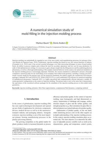
A numerical simulation study of mold filling in the injection molding process5. The results ofthe numerical simulation studyBetween the time steps 0.1 s and 0.2 s the polymermelt contacts the sidewalls of the cavity and the evolutionof a larger flow front can be observed, cf. Figure 10. Thesubsequent filling phase at the time step 0.3 s is characterized by a constant progression of the polymer melt. Itcan be seen that the flow front of the melt is very similarfor all time steps with slight variation in the filling level.Figure 11 shows a temporal shape of the flow frontwithin the mid plane of the cavity. Booth simulation strategies show a good agreement at the evolution of the flowfront. Only on the cavity wall is the melt front slightlydifferent. In Cadmould 3D-F the influence of the boundary conditions is more pronounced than in ANSYS CFX.All simulations were performed on a 3.1 GHz IntelXeon E5-2687W v3 machine with 10 cores / 20 threadsand 32 GBytes RAM. For ANSYS CFX, a multicore(HPC license) 2020 R1 license was employed. For thesimulation in Cadmould 3D-F, a singlecore V13 licensewas used. While the computations in ANSYS CFX werecompleted after 62 hours and 47 minutes, the simulationin Cadmould 3D-F converged in 11 minutes and 31 seconds. The large difference in computation times is mainly caused by the different numerical approaches anddiscretization strategies in ANSYS CFX and Cadmould3D-F. In terms of the simulation of the mold filling, bothsoftware packages provide almost equivalent results.Here, the results in ANSYS CFX serve as a reference forthe validation of Cadmould 3D-F.The simulation results demonstrate that the flowfront of the polymer melt is initially characterizedby the geometry and the inflow process as shown inFigure 9. The comparison is made for the differenttime steps. Due to the 2.5D method in Cadmould3D-F, a smooth flow front is formed. However,ANSYS CFX has slightly sharp edges on the flowfront, which are created by the influence of small eddies at the inlet.Fig. 9. Results for the early filling phase at the time steps0.03 s and 0.05 sa)b)c)d)Fig. 10. Results of the filling phases between the simulations with ANSYS CFX (left) and Cadmould 3D-F (right):a) result at the time step 0.1 s; b) result at the time step 0.2 s; c) result at the time step 0.3 s; d) result at the time step 0.4 s2021, vol. 21, no. 1 31Computer Methods in Materials Science
M. Baum, D. AndersFig. 11. A temporal evolution of the flow front withinthe mid plane of the cavity6. Conclusion and outlookThis contribution demonstrates that the Hele-Shawapproximation employed in the Cadmould 3D-F framework offers a well suited, efficient, and sufficiently accurate simulation of the filling process in thin-walledstructures. The simulation results of the full-volumetric model in ANSYS CFX and the semi-volumetricmodel in Cadmould 3D-F are almost equivalent. Itcan be observed that there are only slight differencesin the contact areas between the polymer melt and thecavity walls. The reason for this can be found in thedifferent setup of the boundary conditions at the walland the characterization of the flow front. In full-volumetric models approaches, the fountain flow regime inthe flow front is captured, while in the semi-volumetric approach, this effect is neglected. Another reasonis that surface tension has certain effects on the flowfront. This has been discussed by Wang et al. (2012).Due to the enormous time savings of calculations inCadmould 3D-F compared to simulations in ANSYSCFX, Cadmould 3D-F may serve as a very efficientsimulation tool for the iterative parameter optimizationin injection molding processes. For the next researchactivities, the authors plan to make further validation ofthe simulation results with experimental filling studiesas well as the implementation of a surrogate-assistedoptimization procedure for injection molding includingsimulations in Cadmould 3D-F.AcknowledgementsThis contribution was developed within theOptiTemp project. The OptiTemp research project(reference number 13FH012PX8) is partly fundedby the German Federal Ministry of Education andResearch (BMBF) within the FHprofUnt 2018 research program.ReferencesCardozo, D. (2009). A brief history of the filling simulation of injection moulding. Journal of Mechanical Engineering Science,223(3), 711–721. https://doi.org/10.1243/09544062JMES986.Chiang, H.H., Hieber, C.A., & Wang, K.K. (1991). A Unified Simulation of the Filling and Postfilling Stages in Injection Molding. Part I: Formulation. Polymer Engineering and Science, 31(2), 116–124. https://doi.org/10.1002/pen.760310210.Fernandez, C., Pontes, A.J., Viana, J.C., & Gaspar-Cunha, A. (2018). Modelling and optimization of the injection-moldingprocess: a review. Advances in Polymer Technology, 37(2), 429–449. https://doi.org/10.1002/adv.21683.Guevara-Morales, A., & Figueroa-López, U. (2014). Residual stresses in injection molded products. Journal of Materials Science, 49, 4399–4415. https://doi.org/10.1007/s10853-014-8170-y.Haagh, G.A.A.V., & Van De Vosse, F.N. (1998). Simulation of three dimensional polymer mould filling processes usinga pseudo concentration method. International Journal for Numerical Methods in Fluids, 28(9), 1355–1369. 8:9 1355::AID-FLD770 3.0.CO;2-C.Hele-Shaw, H.S. (1899). The Motion of a Perfect Liquid. Proceedings of the Royal Institution of Great Britain, 16, 49–64.Hieber, C.A. (1987). Melt viscosity characterization and its application to injection molding. In A.I. Isayev (Ed.), Injection andCompression Molding Fundamentals (pp. 124–129). Marcel Dekker.Hieber, C.A., & Shen, S.F. (1980). A Finite-Element/Finite-Difference Simulation of the Injection-Molding Filling Process.Journal of Non-Newtonian Fluid Mechanics, 7(1), 1–32. r, J.-M., Arab, A., & Stommel, M. (2012). Device to Determine Rheological Properties of Thermoplastics Blended withChemical Foaming Agent. Zeitschrift Kunststofftechnik / Journal of Plastics Technology, 8, 91–105.Karrenberg, G., Neubrech, B., & Wortberg, J. (2013). CFD-Simulation der Kunststoffplastifizierung in einem Extruder mitdurchgehend genutetem Zylinder und Barriereschnecke. Zeitschrift Kunststofftechnik / Journal of Plastics Technology,12(3), 205–238. https://doi.org/10.3139/O999.04032016.Mukras, S.M.S., & Al-Mufadi, F.A (2016). Simulation of HDPE Mold Filling in the Injection Molding Process with Comparison to Experiments. Arabian Journal for Science and Engineering, 41(5), 2847–2856. https://doi.org/10.1007/s13369015-1970-9.Nielsen, L.E., & Landel, R.F. (1994). Mechanical Properties of Polymers and Composites. Marcel Dekker.Osswald, T.A., & Rudolph, N. (2015). Polymer rheology. Fundamentals and applications. Hanser Publications.
A numerical simulation study of mold filling in the injection molding processRezayat, M., & Stafford, R.O. (1991). A thermoviscoelastic model for residual stress in injection molded thermoplastics. Polymer Engineering and Science, 31(6), 393–398. https://doi.org/10.1002/pen.760310602.Rusdi, M.S., Abdullah, M.Z., Mahmud, A.S., Khor, C.Y., Abdul Aziz, M.S., Abdullah, M.K., Yusoff, H., & Firdaus, S.M.(2014). Numerical Investigation on the Effect of Injection Pressure on Melt Front Pressure and Velocity Drop. AppliedMechanics and Material, 786, 210–214. .210.Rusdi, M.S., Abdullah, M.Z., Mahmud, A.S., Khor, C.Y., Abdul Aziz, M.S., Ariff, Z.M., & Abdullah, M.K. (2016). NumericalInvestigation on the Effect of Pressure and Temperature on the Melt Filling During Injection Molding Process. ArabianJournal for Science and Engineering, 41(5), 1907–1919. https://doi.org/10.1007/s13369-016-2039-0.Simcon Kunststofftechnische Software GmbH (2004). Simulation of fluid flow and structural analysis within thin walled threedimensional geometries, European Patent Application, EP 1385103 A1.Studer, M., & Ehring, F. (2013). Reduktion von Formteilverzug beim Spritzgießen durch optimale Wanddickenverteilung –Eine Machbarkeitsstudie. Zeitschrift Kunststofftechnik / Journal of Plastics Technology, 9, 209–252.Studer, M., & Ehring, F. (2014). Minimizing Part Warpage in Injection Molding by Optimizing Wall Thickness Distribution.Advances in Polymer Technology, 33(S1), 21454. https://doi.org/10.1002/adv.21454.Wang, W., Li, X., & Han, X. (2012). Numerical simulation and experimental verification of the filling stage in injection molding. Polymer Engineering and Science, 52(1), 42–51. https://doi.org/10.1002/pen.22043.Zhang, J., Yin, X., Liu, F., & Yang, P. (2016). The simulation of the warpage rule of the thin-walled part of polypropylenecomposite based on the coupling effect of mold deformation and injection molding process. Science and Engineering ofComposite Materials, 25(3), 593–601. https://doi.org/10.1515/secm-2015-0195.
the injection molding process First of all, let us take a closer look at the fundamen - tals of the injection molding process. As illustrated in Figure 2, an injection molding machine can be subdivided into two basic units. In the plasticizing unit, the polymer granulate is fed into the ma