Transcription
Continuum MechanicsVolume II of Lecture Notes onthe Mechanics of SolidsRohan AbeyaratneQuentin Berg Professor of MechanicsMIT Department of Mechanical EngineeringandDirector – SMART CenterSingapore MIT Alliance for Research and TechnologyCopyright c Rohan Abeyaratne, 1988All rights reserved.http://web.mit.edu/abeyaratne/lecture notes.html11 May 2012
3Electronic PublicationRohan AbeyaratneQuentin Berg Professor of MechanicsDepartment of Mechanical Engineering77 Massachusetts Institute of TechnologyCambridge, MA 02139-4307, USACopyright c by Rohan Abeyaratne, 1988All rights reservedAbeyaratne, Rohan, Continuum Mechanics, Volume II of Lecture Notes on the Mechanicsof Solids. / Rohan Abeyaratne – 1st Edition – Cambridge, MA and Singapore:ISBN-13: 978-0-9791865-1-6ISBN-10: 0-9791865-1-XQCPlease send corrections, suggestions and comments to abeyaratne.vol.2@gmail.comUpdated 28 May 2020
4
iDedicated toPods and Nangifor their gifts of love and presence.
iiiNOTE TO READERI had hoped to finalize this second set of notes an year or two after publishing Volume Iof this series back in 2007. However I have been distracted by various other interesting tasksand it has sat on a back-burner. Since I continue to receive email requests for this secondset of notes, I am now making Volume II available even though it is not as yet complete. Inaddition, it has been “cleaned-up” at a far more rushed pace than I would have liked.In the future, I hope to sufficiently edit my notes on Viscoelastic Fluids and Micromechanical Models of Viscoelastic Fluids so that they may be added to this volume; and if Iever get around to it, a chapter on the mechanical response of materials that are affected byelectromagnetic fields.I would be most grateful if the reader would please inform me of any errors in the notesby emailing me at abeyaratne.vol.2@gmail.com.
vPREFACEDuring the period 1986 - 2008, the Department of Mechanical Engineering at MIT offereda series of graduate level subjects on the Mechanics of Solids and Structures that :2.095:2.099:Mechanics of Solid Materials,Mechanics of Continuous Media,Solid Mechanics: Elasticity,Solid Mechanics: Plasticity and Inelastic Deformation,Advanced Mechanical Behavior of Materials,Structural Mechanics,Finite Element Analysis of Solids and Fluids,Molecular Modeling and Simulation for Mechanics, andComputational Mechanics of Materials.Over the years, I have had the opportunity to regularly teach the second and third ofthese subjects, 2.072 and 2.074 (formerly known as 2.083), and the current four volumesare comprised of the lecture notes I developed for them. First drafts of these notes wereproduced in 1987 (Volumes I and IV) and 1988 (Volumes II) and they have been corrected,refined and expanded on every subsequent occasion that I taught these classes. The materialin the current presentation is still meant to be a set of lecture notes, not a text book. It hasbeen organized as follows:Volume I: A Brief Review of Some Mathematical PreliminariesVolume II: Continuum MechanicsVolume III: A Brief Introduction to Finite ElasticityVolume IV: ElasticityThis is Volume II.My appreciation for mechanics was nucleated by Professors Douglas Amarasekara andMunidasa Ranaweera of the (then) University of Ceylon, and was subsequently shaped andgrew substantially under the influence of Professors James K. Knowles and Eli Sternbergof the California Institute of Technology. I have been most fortunate to have had theopportunity to apprentice under these inspiring and distinctive scholars.I would especially like to acknowledge the innumerable illuminating and stimulatinginteractions with my mentor, colleague and friend the late Jim Knowles. His influence on
vime cannot be overstated.I am also indebted to the many MIT students who have given me enormous fulfillmentand joy to be part of their education.I am deeply grateful for, and to, Curtis Almquist SSJE, friend and companion.My understanding of elasticity as well as these notes have benefitted greatly from manyuseful conversations with Kaushik Bhattacharya, Janet Blume, Eliot Fried, Morton E.Gurtin, Richard D. James, Stelios Kyriakides, David M. Parks, Phoebus Rosakis, StewartSilling and Nicolas Triantafyllidis, which I gratefully acknowledge.Volume I of these notes provides a collection of essential definitions, results, and illustrative examples, designed to review those aspects of mathematics that will be encounteredin the subsequent volumes. It is most certainly not meant to be a source for learning thesetopics for the first time. The treatment is concise, selective and limited in scope. For example, Linear Algebra is a far richer subject than the treatment in Volume I, which is limitedto real 3-dimensional Euclidean vector spaces.The topics covered in Volumes II and III are largely those one would expect to see coveredin such a set of lecture notes. Personal taste has led me to include a few special (but stillwell-known) topics. Examples of these include sections on the statistical mechanical theoryof polymer chains and the lattice theory of crystalline solids in the discussion of constitutiverelations in Volume II, as well as several initial-boundary value problems designed to illustratevarious nonlinear phenomena also in Volume II; and sections on the so-called Eshelby problemand the effective behavior of two-phase materials in Volume III.There are a number of Worked Examples and Exercises at the end of each chapter whichare an essential part of the notes. Many of these examples provide more details; or the proofof a result that had been quoted previously in the text; or illustrates a general concept; orestablishes a result that will be used subsequently (possibly in a later volume).The content of these notes are entirely classical, in the best sense of the word, and noneof the material here is original. I have drawn on a number of sources over the years as Iprepared my lectures. I cannot recall every source I have used but certainly they includethose listed at the end of each chapter. In a more general sense the broad approach andphilosophy taken has been influenced by:Volume I: A Brief Review of Some Mathematical PreliminariesI.M. Gelfand and S.V. Fomin, Calculus of Variations, Prentice Hall, 1963.
viiJ.K. Knowles, Linear Vector Spaces and Cartesian Tensors, Oxford University Press,New York, 1997.Volume II: Continuum MechanicsP. Chadwick, Continuum Mechanics: Concise Theory and Problems, Dover,1999.J.L. Ericksen, Introduction to the Thermodynamics of Solids, Chapman and Hall, 1991.M.E. Gurtin, An Introduction to Continuum Mechanics, Academic Press, 1981.M.E. Gurtin, E. Fried and L. Anand, The Mechanics and Thermodynamics of Continua, Cambridge University Press, 2010.J. K. Knowles and E. Sternberg, (Unpublished) Lecture Notes for AM136: Finite Elasticity, California Institute of Technology, Pasadena, CA 1978.C. Truesdell and W. Noll, The nonlinear field theories of mechanics, in Handbüch derPhysik, Edited by S. Flügge, Volume III/3, Springer, 1965.Volume III: ElasticityM.E. Gurtin, The linear theory of elasticity, in Mechanics of Solids - Volume II, editedby C. Truesdell, Springer-Verlag, 1984.J. K. Knowles, (Unpublished) Lecture Notes for AM135: Elasticity, California Instituteof Technology, Pasadena, CA, 1976.A. E. H. Love, A Treatise on the Mathematical Theory of Elasticity, Dover, 1944.S. P. Timoshenko and J.N. Goodier, Theory of Elasticity, McGraw-Hill, 1987.The following notation will be used in Volume II though there will be some lapses (forreasons of tradition): Greek letters will denote real numbers; lowercase boldface Latin letterswill denote vectors; and uppercase boldface Latin letters will denote linear transformations.Thus, for example, α, β, γ. will denote scalars (real numbers); x, y, z, . will denote vectors;and X, Y, Z, . will denote linear transformations. In particular, “o” will denote the nullvector while “0” will denote the null linear transformation.One result of this notational convention is that we will not use the uppercase bold letterX to denote the position vector of a particle in the reference configuration. Instead we usethe lowercase boldface letters x and y to denote the positions of a particle in the referenceand current configurations.
viii
Contents1 Some Preliminary Notions11.1Bodies and Configurations. . . . . . . . . . . . . . . . . . . . . . . . . . . . .21.2Reference Configuration. . . . . . . . . . . . . . . . . . . . . . . . . . . . . .41.3Description of Physical Quantities: Spatial and Referential (or Eulerian andLagrangian) forms. . . . . . . . . . . . . . . . . . . . . . . . . . . . . . . . .61.4Eulerian and Lagrangian Spatial Derivatives. . . . . . . . . . . . . . . . . . .71.5Motion of a Body. . . . . . . . . . . . . . . . . . . . . . . . . . . . . . . . . .91.6Eulerian and Lagrangian Time Derivatives. . . . . . . . . . . . . . . . . . . .101.7A Part of a Body. . . . . . . . . . . . . . . . . . . . . . . . . . . . . . . . . .111.8Extensive Properties and their Densities. . . . . . . . . . . . . . . . . . . . .122 Kinematics: Deformation152.1Deformation . . . . . . . . . . . . . . . . . . . . . . . . . . . . . . . . . . . .2.2Deformation Gradient Tensor. Deformation in the Neighborhood of a Particle. 182.3Some Special Deformations. . . . . . . . . . . . . . . . . . . . . . . . . . . .212.4Transformation of Length, Orientation, Angle, Volume and Area. . . . . . .252.4.1Change of Length and Orientation. . . . . . . . . . . . . . . . . . . .262.4.2Change of Angle. . . . . . . . . . . . . . . . . . . . . . . . . . . . . .272.4.3Change of Volume. . . . . . . . . . . . . . . . . . . . . . . . . . . . .28ix16
xCONTENTS2.4.4Change of Area. . . . . . . . . . . . . . . . . . . . . . . . . . . . . . .292.5Rigid Deformation. . . . . . . . . . . . . . . . . . . . . . . . . . . . . . . . .302.6Decomposition of Deformation Gradient Tensor into a Rotation and a Stretch. 322.7Strain. . . . . . . . . . . . . . . . . . . . . . . . . . . . . . . . . . . . . . . .362.8Linearization. . . . . . . . . . . . . . . . . . . . . . . . . . . . . . . . . . . .392.9Worked Examples and Exercises. . . . . . . . . . . . . . . . . . . . . . . . .423 Kinematics: Motion633.1Motion. . . . . . . . . . . . . . . . . . . . . . . . . . . . . . . . . . . . . . .643.2Rigid Motions. . . . . . . . . . . . . . . . . . . . . . . . . . . . . . . . . . .653.3Velocity Gradient, Stretching and Spin Tensors. . . . . . . . . . . . . . . . .663.4Rate of Change of Length, Orientation, and Volume. . . . . . . . . . . . . .683.4.1Rate of Change of Length and Orientation. . . . . . . . . . . . . . . .683.4.2Rate of Change of Angle. . . . . . . . . . . . . . . . . . . . . . . . . .703.4.3Rate of Change of Volume. . . . . . . . . . . . . . . . . . . . . . . . .713.4.4Rate of Change of Area and Orientation. . . . . . . . . . . . . . . . .713.5Current Configuration as Reference Configuration. . . . . . . . . . . . . . . .743.6Worked Examples and Exercises . . . . . . . . . . . . . . . . . . . . . . . . .783.7Transport Equations. . . . . . . . . . . . . . . . . . . . . . . . . . . . . . . .863.8Change of Observer. Objective Physical Quantities. . . . . . . . . . . . . . .893.9Convecting and Co-Rotating Bases and Rates. . . . . . . . . . . . . . . . . .933.10 Linearization. . . . . . . . . . . . . . . . . . . . . . . . . . . . . . . . . . . .953.11 Worked Examples and Exercises. . . . . . . . . . . . . . . . . . . . . . . . .964 Mechanical Balance Laws and Field Equations4.1101Introduction . . . . . . . . . . . . . . . . . . . . . . . . . . . . . . . . . . . . 102
xiCONTENTS4.2Conservation of Mass. . . . . . . . . . . . . . . . . . . . . . . . . . . . . . . 1044.3Force. . . . . . . . . . . . . . . . . . . . . . . . . . . . . . . . . . . . . . . . 1054.4The Balance of Momentum Principles. . . . . . . . . . . . . . . . . . . . . . 1104.5A Consequence of Linear Momentum Balance: Stress. . . . . . . . . . . . . . 1104.6Field Equations Associated with the Momentum Balance Principles. . . . . . 1144.7Principal Stresses. . . . . . . . . . . . . . . . . . . . . . . . . . . . . . . . . . 1164.8Formulation of Mechanical Principles with Respect to a Reference Configuration.1184.9Stress Power. . . . . . . . . . . . . . . . . . . . . . . . . . . . . . . . . . . . 1254.9.1A Work-Energy Identity. . . . . . . . . . . . . . . . . . . . . . . . . . 1254.9.2Work Conjugate Stress-Strain Pairs. . . . . . . . . . . . . . . . . . . 1264.10 Linearization. . . . . . . . . . . . . . . . . . . . . . . . . . . . . . . . . . . . 1274.11 Objectivity of Mechanical Quantities. . . . . . . . . . . . . . . . . . . . . . . 1284.12 Worked Examples and Exercises. . . . . . . . . . . . . . . . . . . . . . . . . 1295 Thermodynamic Balance Laws and Field Equations1475.1The First Law of Thermodynamics. . . . . . . . . . . . . . . . . . . . . . . . 1475.2The Second Law of Thermodynamics. . . . . . . . . . . . . . . . . . . . . . . 1495.3Formulation of Thermodynamic Principles with Respect to a Reference Configuration. . . . . . . . . . . . . . . . . . . . . . . . . . . . . . . . . . . . . . 1525.4Summary. . . . . . . . . . . . . . . . . . . . . . . . . . . . . . . . . . . . . . 1535.5Objectivity of Thermomechanical Quantities. . . . . . . . . . . . . . . . . . . 1545.6Worked Examples and Exercises. . . . . . . . . . . . . . . . . . . . . . . . . 1586 Singular Surfaces and Jump Conditions1656.1Introduction. . . . . . . . . . . . . . . . . . . . . . . . . . . . . . . . . . . . 1656.2Jump Conditions in 1-D Theory. . . . . . . . . . . . . . . . . . . . . . . . . . 167
xiiCONTENTS6.3Worked Examples and Exercises. . . . . . . . . . . . . . . . . . . . . . . . . 1716.4Kinematic Jump Conditions in 3-D. . . . . . . . . . . . . . . . . . . . . . . . 1736.5Momentum, Energy and Entropy Jump Conditions in 3-D. . . . . . . . . . . 1766.66.5.1Linear Momentum Balance Jump Condition. . . . . . . . . . . . . . . 1766.5.2Summary: Jump Conditions in Lagrangian Formulation. . . . . . . . 1796.5.3Jump Conditions in Eulerian Formulation. . . . . . . . . . . . . . . . 180Worked Examples and Exercises. . . . . . . . . . . . . . . . . . . . . . . . . 1817 Constitutive Principles1937.1Different Functional Forms of Constitutive Response Functions. Some Examples. . . . . . . . . . . . . . . . . . . . . . . . . . . . . . . . . . . . . . . . . 1967.2Illustration. . . . . . . . . . . . . . . . . . . . . . . . . . . . . . . . . . . . . 1988 Thermoelastic Materials2038.1Constitutive Characterization in Primitive Form. . . . . . . . . . . . . . . . 2038.2Implications of the Entropy Inequality. . . . . . . . . . . . . . . . . . . . . . 2048.3Implications of Material Frame Indifference. . . . . . . . . . . . . . . . . . . 2078.4Discussion. . . . . . . . . . . . . . . . . . . . . . . . . . . . . . . . . . . . . . 2098.5Material Symmetry. . . . . . . . . . . . . . . . . . . . . . . . . . . . . . . . . 2138.5.1Some Examples of Material Symmetry Groups. . . . . . . . . . . . . 2178.5.2Imposing Symmetry Requirements on Constitutive Response Functions.2188.6Materials with Internal Constraints. . . . . . . . . . . . . . . . . . . . . . . . 2218.7Some Models of Elastic Materials. . . . . . . . . . . . . . . . . . . . . . . . . 2248.7.1A Compressible Fluid. . . . . . . . . . . . . . . . . . . . . . . . . . . 2248.7.2Neo-Hookean Model. . . . . . . . . . . . . . . . . . . . . . . . . . . . 2258.7.3Blatz-Ko Model. . . . . . . . . . . . . . . . . . . . . . . . . . . . . . 227
CONTENTSxiii8.7.4Gent Model. Limited Extensibility. . . . . . . . . . . . . . . . . . . . 2298.7.5Fung Model for Soft Biological Tissue. . . . . . . . . . . . . . . . . . 2308.8An Elastic Body with One Preferred Direction. . . . . . . . . . . . . . . . . 2318.9Linearized Thermoelasticity. . . . . . . . . . . . . . . . . . . . . . . . . . . . 2348.9.1Linearized Isotropic Thermoelastic Material. . . . . . . . . . . . . . . 2398.10 Worked Examples and Exercises. . . . . . . . . . . . . . . . . . . . . . . . . 2399 Elastic Materials: Micromechanical Models9.19.2Example: Rubber Elasticity.255. . . . . . . . . . . . . . . . . . . . . . . . . . 2569.1.1A Single Long Chain Molecule: A One-Dimensional Toy Model. . . . 2579.1.2A Special Case of the Preceding One-Dimensional Long Chain Molecule.2609.1.3A Single Long Chain Molecule in Three Dimensions. . . . . . . . . . 2639.1.4A Single Long Chain Molecule: Langevin Statistics. . . . . . . . . . . 2659.1.5A Molecular Model for a Generalized Neo-Hookean Material. . . . . . 266Example: Lattice Theory of Elasticity. . . . . . . . . . . . . . . . . . . . . . 2689.2.1A Bravais Lattice. Pair Potential. . . . . . . . . . . . . . . . . . . . . 2699.2.2Homogenous Deformation of a Bravais Lattice. . . . . . . . . . . . . . 2719.2.3Traction and Stress. . . . . . . . . . . . . . . . . . . . . . . . . . . . 2729.2.4Energy. . . . . . . . . . . . . . . . . . . . . . . . . . . . . . . . . . . 2759.2.5Material Frame Indifference. . . . . . . . . . . . . . . . . . . . . . . . 2779.2.6Linearized Elastic Moduli. Cauchy Relations. . . . . . . . . . . . . . 2779.2.7Lattice and Continuum Symmetry. . . . . . . . . . . . . . . . . . . . 2789.2.8Worked Examples and Exercises. . . . . . . . . . . . . . . . . . . . . 28210 Some Nonlinear Effects: Illustrative Examples28710.1 Example (1): Simple Shear. . . . . . . . . . . . . . . . . . . . . . . . . . . . 287
xivCONTENTS10.2 Example (2): Deformation of an Incompressible Cube Under Prescribed Tensile Forces. . . . . . . . . . . . . . . . . . . . . . . . . . . . . . . . . . . . . . 29010.3 Example (3): Growth of a Cavity. . . . . . . . . . . . . . . . . . . . . . . . . 29910.4 Example (4): Inflation of a Thin-Walled Tube. . . . . . . . . . . . . . . . . . 30310.5 Example (5): Nonlinear Wave Propagation. . . . . . . . . . . . . . . . . . . . 31210.6 Worked Examples and Exercises. . . . . . . . . . . . . . . . . . . . . . . . . 31911 Linearized (Thermo)Elasticity32111.1 Linearized Thermoelasticity . . . . . . . . . . . . . . . . . . . . . . . . . . . 32111.1.1 Worked Examples and Exercises . . . . . . . . . . . . . . . . . . . . . 32511.2 Linearized Elasticity: The Purely Mechanical Theory . . . . . . . . . . . . . 32811.2.1 Worked Examples and Exercises . . . . . . . . . . . . . . . . . . . . . 33012 Compressible Fluids. Viscous Fluids.34112.1 Compressible Inviscid Fluids (Elastic Fluids). . . . . . . . . . . . . . . . . . 34212.1.1 Worked Examples and Exercises. . . . . . . . . . . . . . . . . . . . . 34612.1.2 Adiabatic Flows. . . . . . . . . . . . . . . . . . . . . . . . . . . . . . 34812.1.3 Worked Examples and Exercises. . . . . . . . . . . . . . . . . . . . . 34912.2 Incompressible Viscous Fluids. . . . . . . . . . . . . . . . . . . . . . . . . . . 35212.2.1 Example: A Newtonian Fluid. . . . . . . . . . . . . . . . . . . . . . . 35612.2.2 Example: A Generalized Newtonian Fluid. . . . . . . . . . . . . . . . 35712.2.3 Worked Examples and Exercises. . . . . . . . . . . . . . . . . . . . . 35812.2.4 An Important Remark: . . . . . . . . . . . . . . . . . . . . . . . . . . 36612.3 Incompressible Inviscid Fluids. . . . . . . . . . . . . . . . . . . . . . . . . . . 36612.3.1 Worked Examples and Exercises. . . . . . . . . . . . . . . . . . . . . 36713 Liquid Crystals373
CONTENTSxv13.1 Introduction. . . . . . . . . . . . . . . . . . . . . . . . . . . . . . . . . . . . 37313.2 Formulation of basic concepts. . . . . . . . . . . . . . . . . . . . . . . . . . . 37613.3 Reduced Constitutive Relations. . . . . . . . . . . . . . . . . . . . . . . . . . 38313.3.1 Restrictions due to dissipation inequality. . . . . . . . . . . . . . . . . 38313.3.2 Restrictions due to material frame indifference. . . . . . . . . . . . . 38613.3.3 Summary. . . . . . . . . . . . . . . . . . . . . . . . . . . . . . . . . . 38813.4 A Particular Constitutive Model. . . . . . . . . . . . . . . . . . . . . . . . . 38913.4.1 A Free Energy Function ψ: the Frank Energy . . . . . . . . . . . . . 38913.4.2 An Extra Stress τ . . . . . . . . . . . . . . . . . . . . . . . . . . . . . 39013.5 Boundary Conditions: Anchoring. . . . . . . . . . . . . . . . . . . . . . . . . 39113.6 Worked Examples and Exercises. . . . . . . . . . . . . . . . . . . . . . . . . 391
Chapter 1Some Preliminary NotionsIn this preliminary chapter we introduce certain basic notions that underly the continuumtheory of materials. These concepts are essential ingredients of continuum modeling, thoughsometimes they are used implicitly without much discussion. We shall devote some attentionto these notions in this chapter since that will allow for greater clarity in subsequent chapters.For example we frequently speak of an “isotropic material”. Does this mean that thematerial copper, for example, is isotropic? Suppose we have a particular piece of copperthat is isotropic in a given configuration, and we deform it, will it still be isotropic? Whatis isotropy a property of? The material, the body, or the configuration? Speaking of which,what is the difference between a body, a configuration, and a region of space occupied by abody (and is it important to distinguish between them)? . Often we will want to considersome physical property (e.g. the internal energy) associated with a part of a body (i.e. adefinite set of particles of the body). As the body moves through space and this part occupiesdifferent regions of space at different times and the value of this property changes with time,it may be important to be precise about the fact that this property is assigned to a fixedset of particles comprising the part of the body and not the changing region of space that itoccupies. . Or, consider the propagation of a wavefront. Consider a point on the wavefrontand a particle of the body, both of which happen to be located at the same point in spaceat a given instant. However these are distinct entities and at the next instant of time thissame point on the wavefront and particle of the body would no longer be co-located in space.Thus in particular, the velocity of the point of the wavefront is different from the velocityof the particle of the body, even though they are located at the same point in space at thecurrent instant.1
2CHAPTER 1. SOME PRELIMINARY NOTIONSThe concepts introduced in this chapter aim to clarify such issues. We will not be pedantic about these subtleties. Rather, we shall make use of the framework and terminologyintroduced in this chapter only when it helps avoid confusion. The reader is encouragedto pay special attention to the distinctions between the different concepts introduced here.These concepts include the notions ofa body,a configuration of the body,a reference configuration of the body,the region occupied by the body in some configuration,a particle (or material point),the location of a particle in some configuration,a deformation,a motion,Eulerian and Lagrangian descriptions of a physical quantity,Eulerian and Lagrangian spatial derivatives, andEulerian and Lagrangian time derivatives (including the material time derivative).1.1Bodies and Configurations.Our aim is to develop a framework for studying how “objects that occur in nature” respondto the application of forces or other external stimuli. In order to do this, we must constructmathematical idealizations (i.e. mathematical models) of the “objects” and the “stimuli”.Specifically, with regard to the “objects”, we must model their geometric and constitutivecharacter.We shall use the term “body” to be a mathematical abstraction of an “object thatoccurs in nature”. A body B is composed of a set of particles1 p (or material points). In agiven configuration of the body, each particle is located at some definite point y in threedimensional space. The set of all the points in space, corresponding to the locations of allthe particles, is the region R occupied by the body in that configuration. A particular body,composed of a particular set of particles, can adopt different configurations under the action1A particle in continuum mechanics is different to what we refer to as a particle in classical mechanics.For example, a particle in classical mechanics has a mass m 0, while a particle in continuum mechanics isnot endowed with a property called mass.
31.1. BODIES AND CONFIGURATIONS.of different stimuli (forces, heating etc.) and therefore occupy different regions of space underdifferent conditions. Note the distinction between the body, a configuration of the body, andthe region the body occupies in that configuration; we make these distinctions rigorous inwhat follows. Similarly note the distinction between a particle and the position in space itoccupies in some configuration.In order to appreciate the difference between a configuration and the region occupiedin that configuration, consider the following example: suppose that a body, in a certainconfiguration, occupies a circular cylindrical region of space. If the object is “twisted” aboutits axis (as in torsion), it continues to occupy this same (circular cylindrical) region of space.Thus the region occupied by the body has not changed even though we would say that thebody is in a different “configuration”.More formally, in continuum mechanics a body B is a collection of elements which canbe put into one-to-one correspondence with some region R of Euclidean point space2 . Anelement p B is called a particle (or material point). Thus, given a body B, there isnecessarily a mapping χ that takes particles p B into their geometric locations y R inthree-dimensional Euclidean space:y χ(p) where p B, y R.(1.1)The mapping χ is called a configuration of the body B; y is the position occupied by theparticle p in the configuration χ; and R is the region occupied by the body in the configurationχ. Often, we write R χ(B).BRypy χ(p)p χ 1(y)Figure 1.1: A body B that occupies a region R in a configuration χ. A particle p B is located atthe position y R where y χ(p). B is a mathematical abstraction. R is a region in three-dimensionalEuclidean space.2Recall that a “region” is an open connected set. Thus a single particle p does not constitute a body.
4CHAPTER 1. SOME PRELIMINARY NOTIONSSince a configuration χ provides a one-to-one mapping between the particles p and positions y, there is necessarily an inverse mapping χ 1 from R B:p χ 1 (y) where p B, y R.(1.2)Observe that bodies and particles, in the terminology used here, refer to “abstract” entities. Bodies are available to us through their configurations. Actual geometric measurementscan be made on the place occupied by a particle or the region occupied by a body.1.2Reference Configuration.In order to identify a particle of a body, we must label the particles. The abstract particlelabel p, while perfectly acceptable in principle and intuitively clear, is not convenient forcarrying out calculations. It is more convenient to pick some arbitrary configuration of thebody, say χref , and use the (unique) position x χref (p) of a particle in that configurationto label it instead. Such a configuration χref is called a reference configuration of the body.It simply provides a convenient way in which to label the particles of a body. The particlesare now labeled by x instead of p.A second reason for considering a reference configuration is the following: we can studythe geometric characteristics of a configuration χ by studying the geometric properties ofthe points occupying the region R χ(B). This is adequate for modeling certain materials(such as many fluids) where the behavior of the material depends only on the characteristicsof the configuration currently occupied by the body. In describing most solids however oneoften needs to know the changes in geometric characteristics between one configuration andanother configuration (e.g. the change in length, the change in angle etc.). In order todescribe the change in a geometric quantity one must necessarily consider (at least) twoconfigurations of the body: the configuration that one wishes to analyze, and a referenceconfiguration relative to which the changes are to be measured.Let χref and χ be two configurations of a body B and let Rref and R denote the regionsoccupied by the body B in these two configuration; see Figure 1.2. The mappings χref andχ take p x and p y, and likewise B Rref and B R :x χref (p),y χ(p).(1.3)Here p B, x Rref and y R. Thus x and y are the positions of particle p in the twoconfigurations under consideration.
51.2. REFERENCE CONFIGURATION.y y(x) χ(χ 1ref (x))RrefRyRxRrefx χref (p)01x χref (p)p χ 1ref (x)p χ 1ref (x)y y(x) χ(χ 1ref (x))y y(x) χ(χ 1ref (x))R023y χ(p)p χ 1(y)R p R0i F0iBFigure 1.2: A body B that occupies a region R in a configuration χ, and another region Rref in a secondconfiguration χref . A particle p B is located at y χ(p) R in configuration χ, and at x χref (p) Rrefb (x) χ(χ 1in configuration χref . The mapping of Rref R is described by the deformation y yref (x)).b(x) from Rref R:This induces a mapping y ydefb (x) χ(χ 1y yref (x)),x Rref , y R;(1.4)b is called a deformation of the body from the reference configuration χref .yFrequently one picks a particular convenient (usually fixed) reference configuration χrefand studies deformations of the body relative to that configuration. This particular configuration need only be one that the body can sustain, not necessarily one that is actuallysustained in the setting being analyzed. The choice of reference configuration is arbitraryb inin principle (and is usually chosen for reasons of convenience). Note that the function y(1.4) depends on the choice of reference configuration.When working with a single fixed reference configuration, as we will most often do, onecan dispense with talking ab
these subjects, 2.072 and 2.074 (formerly known as 2.083), and the current four volumes are comprised of the lecture notes I developed for them. First drafts of these notes were produced in 1987 (Volumes I and IV) and 1988 (Volumes II) and they have been corrected, re ned and expanded