Transcription
Matrix Theory andLINEAR ALGEBRAAn open text by Peter SelingerBased on the original text by Lyryx Learning and Ken KuttlerCreative Commons License (CC BY)
Matrix Theory and Linear AlgebraAn open text by Peter SelingerBased on the original text by Lyryx Learning and Ken KuttlerFirst editionCONTRIBUTIONSKen Kuttler, Brigham Young UniversityIlijas Farah, York UniversityMarie-Andrée B. Langlois, Dalhousie UniversityPeter Selinger, Dalhousie UniversityLyryx Learning TeamBruce BauslaughPeter ChowNathan FriessStephanie KeyowskiClaude LaflammeMartha LaflammeJennifer MacKenzieTamsyn MurnaghanBogdan SavaLarissa StoneRyan YeeEhsun ZahediCover photography by Pok RieLICENSECreative Commons License (CC BY): This text, including the art and illustrations, are available underthe Creative Commons license (CC BY), allowing anyone to reuse, revise, remix and redistribute the text.To view a copy of this license, visit https:// reative ommons.org/li enses/by/4.0/
Revision historyCurrent revision: Dal 2018 AThis printing: version 487897b of January 10, 2022Extensive edits, additions, and revisions have been completed by Peter Selinger and other contributors.Prior extensive edits, additions, and revisions were made by the editorial staff at Lyryx Learning.All new content (text and images) is released under the same license as noted above. P. Selinger: updated title and front matter.Dal 2018 ADal 2017 B P. Selinger: Extensive revisions and additions. Rewrote most of Chapters 9–11 from scratch.Added application on perspective rendering, error correcting codes, least squares approximationsand curve fitting, an audio demo for Fourier series, sketching of quadratic forms, and principalcomponent analysis. P. Selinger, M.B. Langlois: Re-ordered chapters. Extensive revisions to Chapters 1–8. Addednew sections on fields, cryptography, geometric interpretation of linear transformations, recurrences, systems of linear differential equations. Lyryx: Front matter has been updated including cover, copyright, and revision pages.2017 A2016 B I. Farah: contributed edits and revisions, particularly the proofs in the Properties of DeterminantsII: Some Important Proofs section. Lyryx: The text has been updated with the addition of subsections on Resistor Networks and theMatrix Exponential based on original material by K. Kuttler. Lyryx: New example on Random Walks developed.2016 A2015 A Lyryx: The layout and appearance of the text has been updated, including the title page and newlydesigned back cover. Lyryx: The content was modified and adapted with the addition of new material and severalimages throughout. Lyryx: Additional examples and proofs were added to existing material throughout.2012 A Original text by K. Kuttler of Brigham Young University. That version is used underCreative Commons license CC BY (https:// reative ommons.org/li enses/by/3.0/)made possible by funding from The Saylor Foundation’s Open Textbook Challenge. SeeElementary Linear Algebra for more information and the original version.
ContentsPreface11 Systems of linear equations31.11.2Geometric view of systems of equations . . . . . . . . . . . . . . . . . . . . . . . . . .Algebraic view of systems of equations . . . . . . . . . . . . . . . . . . . . . . . . . . .1.31.41.5Elementary operations . . . . . . . . . . . . . . . . . . . . . . . . . . . . . . . . . . . . 10Gaussian elimination . . . . . . . . . . . . . . . . . . . . . . . . . . . . . . . . . . . . 17Gauss-Jordan elimination . . . . . . . . . . . . . . . . . . . . . . . . . . . . . . . . . . 291.61.7Homogeneous systems . . . . . . . . . . . . . . . . . . . . . . . . . . . . . . . . . . . . 33Uniqueness of the reduced echelon form . . . . . . . . . . . . . . . . . . . . . . . . . . 381.81.9Fields . . . . . . . . . . . . . . . . . . . . . . . . . . . . . . . . . . . . . . . . . . . . . 42Application: Balancing chemical reactions . . . . . . . . . . . . . . . . . . . . . . . . . 511.101.11Application: Dimensionless variables . . . . . . . . . . . . . . . . . . . . . . . . . . . . 53Application: Resistor networks . . . . . . . . . . . . . . . . . . . . . . . . . . . . . . . 562 Vectors in Rn37612.12.2Points and vectors . . . . . . . . . . . . . . . . . . . . . . . . . . . . . . . . . . . . . . 61Addition . . . . . . . . . . . . . . . . . . . . . . . . . . . . . . . . . . . . . . . . . . . 652.32.42.5Scalar multiplication . . . . . . . . . . . . . . . . . . . . . . . . . . . . . . . . . . . . . 69Linear combinations . . . . . . . . . . . . . . . . . . . . . . . . . . . . . . . . . . . . . 71Length of a vector . . . . . . . . . . . . . . . . . . . . . . . . . . . . . . . . . . . . . . 752.6The dot product . . . . . . . . . . . . . . . . . . . . . . . . . . . . . . . . . . . . . . . 792.6.1 Definition and properties . . . . . . . . . . . . . . . . . . . . . . . . . . . . . . . 802.6.22.6.32.7The Cauchy-Schwarz and triangle inequalities . . . . . . . . . . . . . . . . . . . . 81The geometric significance of the dot product . . . . . . . . . . . . . . . . . . . . 822.6.4 Orthogonal vectors . . . . . . . . . . . . . . . . . . . . . . . . . . . . . . . . . . 842.6.5 Projections . . . . . . . . . . . . . . . . . . . . . . . . . . . . . . . . . . . . . . 84The cross product . . . . . . . . . . . . . . . . . . . . . . . . . . . . . . . . . . . . . . 902.7.12.7.2Right-handed systems of vectors . . . . . . . . . . . . . . . . . . . . . . . . . . . 90Geometric description of the cross product . . . . . . . . . . . . . . . . . . . . . 912.7.32.7.4Algebraic definition of the cross product . . . . . . . . . . . . . . . . . . . . . . . 92The box product . . . . . . . . . . . . . . . . . . . . . . . . . . . . . . . . . . . 95v
viCONTENTS3 Lines and planes in Rn1013.1Lines . . . . . . . . . . . . . . . . . . . . . . . . . . . . . . . . . . . . . . . . . . . . . 1013.2Planes . . . . . . . . . . . . . . . . . . . . . . . . . . . . . . . . . . . . . . . . . . . . 1104 Matrices1214.1Definition and equality . . . . . . . . . . . . . . . . . . . . . . . . . . . . . . . . . . . 1214.2Addition . . . . . . . . . . . . . . . . . . . . . . . . . . . . . . . . . . . . . . . . . . . 1234.34.4Scalar multiplication . . . . . . . . . . . . . . . . . . . . . . . . . . . . . . . . . . . . . 126Matrix multiplication . . . . . . . . . . . . . . . . . . . . . . . . . . . . . . . . . . . . 1284.4.14.4.24.54.6Multiplying a matrix and a vector . . . . . . . . . . . . . . . . . . . . . . . . . . 128Matrix multiplication . . . . . . . . . . . . . . . . . . . . . . . . . . . . . . . . . 1314.4.3 Properties of matrix multiplication . . . . . . . . . . . . . . . . . . . . . . . . . . 137Matrix inverses . . . . . . . . . . . . . . . . . . . . . . . . . . . . . . . . . . . . . . . . 1424.5.14.5.24.5.3Definition and uniqueness . . . . . . . . . . . . . . . . . . . . . . . . . . . . . . 142Computing inverses . . . . . . . . . . . . . . . . . . . . . . . . . . . . . . . . . . 143Using the inverse to solve a system of equations . . . . . . . . . . . . . . . . . . . 1474.5.44.5.5Properties of the inverse . . . . . . . . . . . . . . . . . . . . . . . . . . . . . . . 148Right and left inverses . . . . . . . . . . . . . . . . . . . . . . . . . . . . . . . . 148Elementary matrices . . . . . . . . . . . . . . . . . . . . . . . . . . . . . . . . . . . . . 1534.6.1 Elementary matrices and row operations . . . . . . . . . . . . . . . . . . . . . . . 1534.6.24.6.34.6.4Inverses of elementary matrices . . . . . . . . . . . . . . . . . . . . . . . . . . . 155Elementary matrices and reduced echelon forms . . . . . . . . . . . . . . . . . . 156Writing an invertible matrix as a product of elementary matrices . . . . . . . . . . 1584.74.6.5 More properties of inverses . . . . . . . . . . . . . . . . . . . . . . . . . . . . . . 159The transpose . . . . . . . . . . . . . . . . . . . . . . . . . . . . . . . . . . . . . . . . 1624.84.9Matrix arithmetic modulo p . . . . . . . . . . . . . . . . . . . . . . . . . . . . . . . . . 165Application: Cryptography . . . . . . . . . . . . . . . . . . . . . . . . . . . . . . . . . 1675 Spans, linear independence, and bases in Rn5.15.25.3175Spans . . . . . . . . . . . . . . . . . . . . . . . . . . . . . . . . . . . . . . . . . . . . . 175Linear independence . . . . . . . . . . . . . . . . . . . . . . . . . . . . . . . . . . . . . 1795.2.15.2.2Redundant vectors and linear independence . . . . . . . . . . . . . . . . . . . . . 179The casting-out algorithm . . . . . . . . . . . . . . . . . . . . . . . . . . . . . . 1815.2.35.2.45.2.5Alternative characterization of linear independence . . . . . . . . . . . . . . . . . 182Properties of linear independence . . . . . . . . . . . . . . . . . . . . . . . . . . 185Linear independence and linear combinations . . . . . . . . . . . . . . . . . . . . 1865.2.6 Removing redundant vectors . . . . . . . . . . . . . . . . . . . . . . . . . . . . . 187Subspaces of Rn . . . . . . . . . . . . . . . . . . . . . . . . . . . . . . . . . . . . . . . 190
CONTENTS5.4Basis and dimension . . . . . . . . . . . . . . . . . . . . . . . . . . . . . . . . . . . . . 1945.4.1 Definition of basis . . . . . . . . . . . . . . . . . . . . . . . . . . . . . . . . . . 1955.4.25.4.35.4.45.5viiExamples of bases . . . . . . . . . . . . . . . . . . . . . . . . . . . . . . . . . . 196Bases and coordinate systems . . . . . . . . . . . . . . . . . . . . . . . . . . . . 198Dimension . . . . . . . . . . . . . . . . . . . . . . . . . . . . . . . . . . . . . . 2005.4.5 More properties of bases and dimension . . . . . . . . . . . . . . . . . . . . . . . 202Column space, row space, and null space of a matrix . . . . . . . . . . . . . . . . . . . . 2106 Linear transformations in Rn2176.16.2Linear transformations . . . . . . . . . . . . . . . . . . . . . . . . . . . . . . . . . . . . 217The matrix of a linear transformation . . . . . . . . . . . . . . . . . . . . . . . . . . . . 2206.36.4Geometric interpretation of linear transformations . . . . . . . . . . . . . . . . . . . . . 225Properties of linear transformations . . . . . . . . . . . . . . . . . . . . . . . . . . . . . 2306.5Application: Perspective rendering . . . . . . . . . . . . . . . . . . . . . . . . . . . . . 2357 Determinants2417.1Determinants of 2 2- and 3 3-matrices . . . . . . . . . . . . . . . . . . . . . . . . . 2417.2Minors and cofactors . . . . . . . . . . . . . . . . . . . . . . . . . . . . . . . . . . . . 2437.37.4The determinant of a triangular matrix . . . . . . . . . . . . . . . . . . . . . . . . . . . 248Determinants and row operations . . . . . . . . . . . . . . . . . . . . . . . . . . . . . . 2507.57.6Properties of determinants . . . . . . . . . . . . . . . . . . . . . . . . . . . . . . . . . . 253Application: A formula for the inverse of a matrix . . . . . . . . . . . . . . . . . . . . . 2587.7Application: Cramer’s rule . . . . . . . . . . . . . . . . . . . . . . . . . . . . . . . . . 2668 Eigenvalues, eigenvectors, and diagonalization2698.1Eigenvectors and eigenvalues . . . . . . . . . . . . . . . . . . . . . . . . . . . . . . . . 2698.28.38.4Finding eigenvalues . . . . . . . . . . . . . . . . . . . . . . . . . . . . . . . . . . . . . 273Geometric interpretation of eigenvectors . . . . . . . . . . . . . . . . . . . . . . . . . . 281Diagonalization . . . . . . . . . . . . . . . . . . . . . . . . . . . . . . . . . . . . . . . 2848.58.6Application: Matrix powers . . . . . . . . . . . . . . . . . . . . . . . . . . . . . . . . . 290Application: Solving recurrences . . . . . . . . . . . . . . . . . . . . . . . . . . . . . . 2938.7Application: Systems of linear differential equations . . . . . . . . . . . . . . . . . . . . 2998.7.1 Differential equations . . . . . . . . . . . . . . . . . . . . . . . . . . . . . . . . . 2998.7.28.7.38.88.98.10Systems of linear differential equations . . . . . . . . . . . . . . . . . . . . . . . 300Example: coupled train cars . . . . . . . . . . . . . . . . . . . . . . . . . . . . . 302Application: The matrix exponential . . . . . . . . . . . . . . . . . . . . . . . . . . . . 308Properties of eigenvectors and eigenvalues . . . . . . . . . . . . . . . . . . . . . . . . . 311The Cayley-Hamilton Theorem . . . . . . . . . . . . . . . . . . . . . . . . . . . . . . . 315
viiiCONTENTS8.11Complex eigenvalues and eigenvectors . . . . . . . . . . . . . . . . . . . . . . . . . . . 3179 Vector spaces3259.1Definition of vector spaces . . . . . . . . . . . . . . . . . . . . . . . . . . . . . . . . . 3259.29.39.4Linear combinations, span, and linear independence . . . . . . . . . . . . . . . . . . . . 334Subspaces . . . . . . . . . . . . . . . . . . . . . . . . . . . . . . . . . . . . . . . . . . 342Basis and dimension . . . . . . . . . . . . . . . . . . . . . . . . . . . . . . . . . . . . . 3499.5Application: Error correcting codes . . . . . . . . . . . . . . . . . . . . . . . . . . . . . 35510 Linear transformation of vector spaces36910.1 Definition and examples . . . . . . . . . . . . . . . . . . . . . . . . . . . . . . . . . . . 36910.210.3The algebra of linear transformations . . . . . . . . . . . . . . . . . . . . . . . . . . . . 375Linear transformations defined on a basis . . . . . . . . . . . . . . . . . . . . . . . . . . 37810.4The matrix of a linear transformation . . . . . . . . . . . . . . . . . . . . . . . . . . . . 38111 Inner product spaces38711.1 Real inner product spaces . . . . . . . . . . . . . . . . . . . . . . . . . . . . . . . . . . 38711.211.3Orthogonality . . . . . . . . . . . . . . . . . . . . . . . . . . . . . . . . . . . . . . . . 394The Gram-Schmidt orthogonalization procedure . . . . . . . . . . . . . . . . . . . . . . 40311.411.511.6Orthogonal projections and Fourier series . . . . . . . . . . . . . . . . . . . . . . . . . . 413Application: Least squares approximations and curve fitting . . . . . . . . . . . . . . . . 424Orthogonal functions and orthogonal matrices . . . . . . . . . . . . . . . . . . . . . . . 43211.711.8Diagonalization of symmetric matrices . . . . . . . . . . . . . . . . . . . . . . . . . . . 437Positive semidefinite and positive definite matrices . . . . . . . . . . . . . . . . . . . . . 44211.9 Application: Simplification of quadratic forms . . . . . . . . . . . . . . . . . . . . . . . 44811.10 Complex inner product spaces . . . . . . . . . . . . . . . . . . . . . . . . . . . . . . . . 45611.11 Unitary and hermitian matrices . . . . . . . . . . . . . . . . . . . . . . . . . . . . . . . 46611.12 Application: Principal component analysis . . . . . . . . . . . . . . . . . . . . . . . . . 472A Complex numbersA.1A.2A.3485The complex numbers . . . . . . . . . . . . . . . . . . . . . . . . . . . . . . . . . . . . 485Geometric interpretation . . . . . . . . . . . . . . . . . . . . . . . . . . . . . . . . . . . 489The fundamental theorem of algebra . . . . . . . . . . . . . . . . . . . . . . . . . . . . 491B Answers to selected exercises495Index541
PrefaceMatrix Theory and Linear Algebra is an introduction to linear algebra for students in the first or secondyear of university. The book contains enough material for a 2-semester course. Major topics of linearalgebra are presented in detail, and many applications are given. Although it is not a proof-oriented book,proofs of most important theorems are provided.Each section begins with a list of desired outcomes which a student should be able to achieve uponcompleting the chapter. Throughout the text, examples and diagrams are given to reinforce ideas andprovide guidance on how to approach various problems. Students are encouraged to work through thesuggested exercises provided at the end of each section. Selected solutions to these exercises are given atthe end of the text.Open textThis is an open text, licensed under the Creative Commons “CC BY 4.0” license. This means, amongother things, that you are permitted to copy and redistribute this textbook in any medium or format. Forexample, you can download this textbook for free, print copies for yourself or others, or share it on theinternet.The license also permits making changes. This is ideal for instructors who would like to add theirown material, change notations, or add more examples or exercises. If you make revisions, pleasesend them to me so that I can consider incorporating them in future versions of this book. Please seehttps:// reative ommons.org/li enses/by/4.0/ for details of the licensing terms.This textbook has a website at https://www.mathstat.dal. a/ selinger/linear-algebra/ .There, you can find the most up-to-date version. The website also contains supplementary material, a linkto the source code and license, options for purchasing a printed version of this book, and more.Reporting typosLike all books, this book likely contains some typos and other errors. However, since it is an open text,typos can easily be fixed and an updated version posted online. It is my intention to fix all typos. Ifyou find a typo (no matter how small), please report it to me at selinger@mathstat.dal.ca. Thanks to thefollowing people who have already reported typos: Yaser Alkayale, Hassaan Asif, Courtney Baumgartner,Kieran Bhaskara, Serena Drouillard, Robert Earle, Warren Fisher, Esa Hannila, Melissa Huggan, XiaoyuJia, Arman Kerimbek, Peter Lake, Marie-Andrée Langlois, Brenda Le, Sarah Li, Ian MacIntosh, Li WeiMen, Deklan Mengering, Dallas Sawtell, Alain Schaerer, Yi Shu, Bruce Smith, Asmita Sodhi, Michael StDenis, Daniele Turchetti, Liu Yuhao, and Ziqi Zhang.1
1. Systems of linear equations1.1 Geometric view of systems of equationsOutcomesA. Relate the types of solution sets of a system of two (three) variables to the intersections oflines in a plane (the intersection of planes in 3-dimensional space)As you may remember, linear equations like 2x 3y 6 can be graphed as straight lines in the coordinateplane. We say that this equation is in two variables, in this case x and y. Suppose you have two suchequations, each of which can be graphed as a straight line, and consider the resulting graph of two lines.What would it mean if there exists a point of intersection between the two lines? This point, which lieson both graphs, gives x and y values for which both equations are true. In other words, this point gives theordered pair (x, y) that satisfies both equations. If the point (x, y) is a point of intersection, we say that (x, y)is a solution to the two equations. In linear algebra, we often are concerned with finding the solution(s)to a system of equations, if such solutions exist. First, we consider graphical representations of solutionsand later we will consider the algebraic methods for finding solutions.When looking for the intersection of two lines in the plane, several situations may arise. The following picture demonstrates the possible situations when considering two equations (two lines in the plane)involving two variables.yxOne solutionyyxNo solutionsxInfinitely many solutionsIn the first diagram, there is a unique point of intersection, which means that there is only one (unique)solution to the two equations. In the second, there are no points of intersection and no solution. There isno solution because the two lines are parallel and they never intersect. The third situation that can occur,as demonstrated in diagram three, is that the two lines are really the same line. For example, x y 1and 2x 2y 2 are two equations that yield the same line when graphed. In this case there are infinitelymany points that are solutions of these two equations, as every ordered pair which is on the graph of theline satisfies both equations.When considering linear systems of equations, there are always three possibilities for the number ofsolutions: there is exactly one solution, there are infinitely many solutions, or there is no solution. When3
4Systems of linear equationswe speak of solving a system of equations, we usually mean finding all of its solutions. This can meanfinding one solution (if the solution is unique), finding infinitely many solutions, or finding that there is nosolution.Example 1.1: A graphical solutionUse a graph to solve the following system of equations:x y 3y x 5.Solution. Through graphing the above equations and identifying the point of intersection, we can find thesolution(s). Remember that we must have either one solution, infinitely many, or no solutions at all. Thefollowing graph shows the two equations, as well as the intersection. Remember, the point of intersectionrepresents the solution of the two equations, or the (x, y) which satisfy both equations. In this case, thereis one point of intersection at ( 1, 4) which means we have one unique solution, x 1, y 4.yy x 565(x, y) ( 1, 4)43x y 321x 4 3 2 11 In the above example, we investigated the intersection point of two equations in two variables, x and y.Now we will consider the graphical solutions of three equations in two variables.Consider a system of three equations in two variables. Again, these equations can be graphed asstraight lines in the plane, so that the resulting graph contains three straight lines. Recall the three possibilities for the number of solutions: no solution, one solution, and infinitely many solutions. With threelines, there are more complex ways of achieving these situations. For example, you can imagine the caseof three intersecting lines having no common point of intersection. Perhaps you can also imagine threeintersecting lines which do intersect at a single point. These two situations are illustrated below.yyxNo solutionxOne solution
1.1. Geometric view of systems of equations5Consider the first picture above. While all three lines intersect with one another, there is no commonpoint of intersection where all three lines meet at one point. Hence, there is no solution to the threeequations. Remember, a solution is a point (x, y) which satisfies all three equations. In the case of thesecond picture, the lines intersect at a common point. This means that there is one solution to the threeequations whose graphs are the given lines. You should take a moment now to draw the graph of a systemwhich results in three parallel lines. Next, try the graph of three identical lines. Which type of solution isrepresented in each of these graphs?We have now considered the graphical solutions of systems of two equations in two variables, as wellas three equations in two variables. However, there is no reason to limit our investigation to equations intwo variables. We will now consider equations in three variables.You may recall that equations in three variables, such as 2x 4y 5z 8, form a plane. Above, wewere looking for intersections of lines in order to identify any possible solutions. When graphically solvingsystems of equations in three variables, we look for intersections of planes. These points of intersectiongive the (x, y, z) that satisfy all the equations in the system. What types of solutions are possible whenworking with three variables? Consider the following picture involving two planes, which are given bytwo equations in three variables.Notice how these two planes intersect in a line. This means that the points (x, y, z) on this line satisfyboth equations in the system. Since the line contains infinitely many points, this system has infinitelymany solutions.It could also happen that the two planes fail to intersect. However, is it possible to have two planesintersect at a single point? Take a moment to attempt drawing this situation, and convince yourself that itis not possible! This means that when we have only two equations in three variables, there is no way tohave a unique solution! Hence, the only possibilities for the number of solutions of two equations in threevariables are no solution or infinitely many solutions.Now imagine adding a third plane. In other words, consider three equations in three variables. Whattypes of solutions are now possible? Consider the following diagram.
6Systems of linear equationsIn this diagram, there is no point which lies in all three planes. There is no intersection between allthree planes so there is no solution. The picture illustrates the situation in which the line of intersectionof the new plane with one of the original planes forms a line parallel to the line of intersection of the firsttwo planes. However, in three dimensions, it is possible for two lines to fail to intersect even though theyare not parallel. Such lines are called skew lines.Recall that when working with two equations in three variables, it was not possible to have a uniquesolution. Is it possible when considering three equations in three variables? In fact, it is possible, and wedemonstrate this situation in the following picture.In this case, the three planes have a single point of intersection. Can you think of other possibilities?Another is that the three planes could intersect in a line, resulting in infinitely many solutions, as in thefollowing diagram.We have now seen how three equations in three variables can have no solution, a unique solution, orintersect in a line resulting in infinitely many solutions. It is also possible that all three equations describethe same plane, which also leads to infinitely many solutions.You can see that when working with equations in three variables, there are many more possibilities forachieving solutions (or no solutions) than when working with two variables. It may prove enlightening tospend time imagining (and drawing) many possible scenarios, and you should take some time to try a few.You should also take some time to imagine (and draw) graphs of systems in more than three variables.Equations like x y 2z 4w 8 with more than three variables are often called hyperplanes. Youmay soon realize that it is tricky to draw the graphs of hyperplanes! In fact, most people cannot visualizemore than three dimensions. Fortunately, through the tools of linear algebra, we can examine systemsof equations in four variables, five variables, or even hundreds or thousands of variables, without everneeding to graph them. Instead we will use algebra to manipulate and solve these systems of equations.We will introduce these algebraic tools in the following sections.
1.2. Algebraic view of systems of equations7ExercisesExercise 1.1.1 Graphically, find the point (x, y) which lies on both of the lines x 3y 1 and 4x y 3.That is, graph each line and see where they intersect.Exercise 1.1.2 Graphically, find the point of intersection of the two lines 3x y 3 and x 2y 1. Thatis, graph each line and see where they intersect.Exercise 1.1.3 You have a system of k equations in two variables, k 2. Explain the geometric significance of(a) No solution.(b) A unique solution.(c) An infinite number of solutions.Exercise 1.1.4 Draw a picture of three planes such that no two of the planes are parallel, but the threeplanes have no common intersection.1.2 Algebraic view of systems of equationsOutcomesA. Recognize the difference between a linear equation and a non-linear equation.B. Determine whether a tuple of real numbers is a solution for a system of linear equations.C. Understand what it means for a system of linear equations to be consistent or inconsistent.We have taken an in-depth look at graphical representations of systems of equations, as well as how tofind possible solutions graphically. Our attention now turns to working with systems algebraically.Definition 1.2: Linear equationA linear equation is an equation of the forma1 x1 a2 x2 . . . an xn b.Here, a1 , . . . , an are real numbers called the coefficients of the equation, b is a real number calledthe constant term of the equation, and x1 , . . . , xn are variables.
8Systems of linear equationsReal numbers, such as the coefficients a1 , . . . , an , the constant term b, or the values of the variablesx1 , . . . , xn , will also be called scalars. For now, the word “scalar” is just a synonym for “real number”.Later, in Section 1.8, we will discover other kinds of scalars.Example 1.3: Linear vs. non-linear equationWhich of the following equations are linear?2x 3y 522x 3y 52 x 3y 5 ( 2)x 3y 522 3y 5 is not linear, because it containsSolution. The equation 2x 3y 5 is linear. The equation 2x the square of a variable instead of a variable. The equation 2 x 3y 5 is alsothe not linear, because2square root is applied to one of the variables. On the other hand, the equation ( 2)x 3y 5 is linear,because 2 and 52 are real numbers, and can therefore be used as coefficients and constant terms. We also permit minor notational variants of linear equations. The equation 2x 3y 5 is linear althoughDefinition 1.2 does not mention subtraction, because it can be regarded as just another notation for 2x ( 3)y 5. Similarly, the equation 2x 5 3y can be regarded as linear, because it can be easily rewrittenas 2x 3y 5 by bringing all the variables (and their coefficients) to the left-hand side. When we need toemphasize that some linear equation is literally of the form a1 x1 a2 x2 . . . an xn b, we say that theequation is in standard form. Thus, the standard form of the equation 2x 5 3y is 2x ( 3)y 5.A solution to a linear equation is an assignment of real numbers to the variables, making the equationtrue. More precisely, if r1 , . . . , rn are real numbers, the assignment x1 r1 , . . . , xn rn is a solution to theequation in Definition 1.2 if the real number a1 r1 a2 r2 . . . an rn is equal to the real number b. To savespace, we often write solutions in tuple notation1 as (x1 , . . . , xn ) (r1 , . . . , rn ). When there is no doubtabout the order of the variables, we also often simply write the solution as (r1 , . . . , rn ).Example 1.4: Solutions of a linear equationConsider the linear equation 2x 3y 4z 5. Which of the following are solutions? (a) (x, y, z) (1, 1, 0), (b) (x, y,
year of university. The book contains enough material for a 2-semester course. Major topics of linear algebra are presented in detail, and many applications are given. Although it is not a proof-oriented book, proofs of most important theorems are provided. Each section begins with a list