WIXLIB

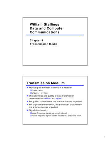
BASIC LINEAR DESIGN Is far less sensitive to load-matching, requiring neither diplexer nor broadbandtermination.Using appropriate design techniques it can provide trade-offs between third-orderintercept (3OI or IP3) and the 1 dB gain-compression point (P1dB), on the one hand, andtotal power consumption (PD) on the other. (That is, including the LO power, which in apassive mixer is hidden in the drive circuitry.)Basic Operation of the Active MixerUnlike the diode-ring mixer, which performs the polarity-reversing switching function inthe voltage domain, the active mixer performs the switching function in the currentdomain. Thus the active mixer core (transistors Q3 through Q6 in Figure 4.8) must bedriven by current-mode signals. The voltage-to-current converter formed by Q1 and Q2receives the voltage-mode RF signal at their base terminals and transforms it into adifferential pair of currents at their collectors.IF OUTPUTQ3Q4Q6Q5LOINPUTQ1Q2RFINPUTIEEFigure 4.8: Classic Active MixerA second point of difference between the active mixer and diode ring mixer, therefore, isthat the active mixer responds only to magnitude of the input voltage, not to the inputpower; that is, the active mixer is not matched to the source. (The concept of matching isthat both the current and the voltage at some port are used by the circuitry which formsthat port). By altering the bias current, IEE, the transconductance of the input pair Q1–Q24.8

RF/IF CIRCUITSMIXERcan be set over a wide range. Using this capability, an active mixer can provide variablegain.A third point of difference is that the output (at the collectors of Q3–Q6) is in the form ofa current, and can be converted back to a voltage at some other impedance level to thatused at the input, hence, can provide further gain. By combining both output currents(typically, using a transformer) this voltage gain can be doubled. Finally, it will beapparent that the isolation between the various ports, in particular, from the LO port tothe RF port, is inherently much lower than can be achieved in the diode ring mixer, dueto the reversed-biased junctions that exist between the ports.Briefly stated, though, the operation is as follows. In the absence of any voltagedifference between the bases of Q1 and Q2, the collector currents of these two transistorsare essentially equal. Thus, a voltage applied to the LO input results in no change ofoutput current. Should a small dc offset voltage be present at the RF input (due typicallyto mismatch in the emitter areas of Q1 and Q2), this will only result in a smallfeedthrough of the LO signal to the IF output, which will be blocked by the first IF filter.Conversely, if an RF signal is applied to the RF port, but no voltage difference is appliedto the LO input, the output currents will again be balanced. A small offset voltage (duenow to emitter mismatches in Q3–Q6) may cause some RF signal feedthrough to the IFoutput; as before, this will be rejected by the IF filters. It is only when a signal is appliedto both the RF and LO ports that a signal appears at the output; hence, the term doublybalanced mixer.Active mixers can realize their gain in one other way: The matching networks used totransform a 50 Ω source to the (usually) high input impedance of the mixer provides animpedance transformation and thus voltage gain due to the impedance step up. Thus, anactive mixer that has loss when the input is terminated in a broadband 50 Ω terminationcan have “gain” when an input matching network is used.4.9

BASIC LINEAR DESIGNREFERENCES:1.Barrie Gilbert, ISSCC Digest of Technical Papers 1968, pp. 114-115, February 16, 1968.2.Barrie Gilbert, Journal of Solid State Circuits, Vol. SC-3, December 1968, pp. 353-372.3.C.L. Ruthroff, Some Broadband Transformers, Proc. I.R.E., Vol.47, August, 1959,pp.1337-1342.4.James M. Bryant, Mixers for High Performance Radio, Wescon 1981: Session 24 (Published byElectronic Conventions, Inc., Sepulveda Blvd., El Segundo, CA)5.P.E. Chadwick, High Performance IC Mixers, IERE Conference on Radio Receivers andAssociated Systems, Leeds, 1981, IERE Conference Publication No. 50.6.P.E. Chadwick, Phase Noise, Intermodulation, and Dynamic Range, RF Expo, Anaheim, CA,January, 1986.7.AD831 Data Sheet, Rev. B, Analog Devices.4.10

RF/IF CIRCUITSMODULATORSECTION 4.2: MODULATORSModulators (sometimes called balanced-modulators, doubly-balanced modulators oreven on occasions high level mixers) can be viewed as sign-changers. The two inputs, Xand Y, generate an output W, which is simply one of these inputs (say, Y) multiplied byjust the sign of the other (say, X), that is W Y* sign (X). Therefore, no referencevoltage is required. A good modulator exhibits very high linearity in its signal path, withprecisely equal gain for positive and negative values of Y, and precisely equal gain forpositive and negative values of X. Ideally, the amplitude of the X input needed to fullyswitch the output sign is very small, that is, the X-input exhibits a comparator-likebehavior. In some cases, where this input may be a logic signal, a simpler X-channel canbe used.As an example, the AD8345 is a silicon RFIC quadrature modulator, designed for usefrom 250 MHz to 1000 MHz. Its excellent phase accuracy and amplitude balance enablethe high performance direct modulation of an IF carrier.The AD8345 accurately splits the external LO signal into two quadrature componentsthrough the polyphase phase-splitter network. The two I and Q LO components are mixedwith the baseband I and Q differential input signals. Finally, the outputs of the twomixers are combined in the output stage to provide a single-ended 50 Ω drive at VOUT.Figure 4.9: AD8345 Block Diagram4.11

BASIC LINEAR DESIGNNotes:4.12

RF/IF CIRCUITSANALOG MULTIPLIERSSECTION 4.3: ANALOG MULTIPLIERSA multiplier is a device having two input ports and an output port. The signal at theoutput is the product of the two input signals. If both input and output signals arevoltages, the transfer characteristic is the product of the two voltages divided by a scalingfactor, K, which has the dimension of voltage (see Figure 4.10). From a mathematicalpoint of view, multiplication is a four quadrant operation—that is to say that both inputsmay be either positive or negative and the output can be positive or negative. Some of thecircuits used to produce electronic multipliers, however, are limited to signals of onepolarity. If both signals must be unipolar, we have a single quadrant multiplier, and theoutput will also be unipolar. If one of the signals is unipolar, but the other may haveeither polarity, the multiplier is a two quadrant multiplier, and the output may have eitherpolarity (and is bipolar). The circuitry used to produce one- and two-quadrant multipliersmay be simpler than that required for four quadrant multipliers, and since there are manyapplications where full four quadrant multiplication is not required, it is common to findaccurate devices which work only in one or two quadrants. An example is the AD539, awideband dual two-quadrant multiplier which has a single unipolar Vy input with arelatively limited bandwidth of 5 MHz, and two bipolar Vx inputs, one per multiplier,with bandwidths of 60 MHz. A block diagram of the AD539 is shown in Figure 4.12.VxV out VxVyVyKK SCALE FACTORFigure 4.10: An Analog Multiplier Block DiagramTypeVXVYVoutSingle QuadrantUnipolarUnipolarUnipolarTwo QuadrantBipolarUnipolarBipolarFour QuadrantBipolarBipolarBipolarFigure 4.11: Definition of Multiplier Quadrants4.13

BASIC LINEAR DESIGNZ1W1VX1VW1 CH1MULTCH2MULT-VX1 VYEXTERNALOP AMPSVYVW2 VX2-VX2 VYW2Z2Figure 4.12: AD539 Block DiagramThe simplest electronic multipliers use logarithmic amplifiers. The computation relies onthe fact that the antilog of the sum of the logs of two numbers is the product of thosenumbers (see Figure 4.13).XLOG YANTILOGXYANTILOGXYLOGMULTIPLICATIONXLOG YLOGDIVISIONXLOGXAANTILOGXRAISING TO A POWER AFigure 4.13: Multiplication Using Log Amps4.14A

RF/IF CIRCUITSANALOG MULTIPLIERSThe disadvantages of this type of multiplication are the very limited bandwidth and singlequadrant operation. A far better type of multiplier uses the Gilbert Cell. This structurewas invented by Barrie Gilbert, now of Analog Devices, in the late 1960s. (SeeReferences 1 and 2).There is a linear relationship between the collector current of a silicon junction transistorand its transconductance (gain) which is given byEq. 4-5dIc / dVbe qIc / kTwhereIc the collector currentVbe the base-emitter voltageq the electron charge (1.60219x10-19)k Boltzmann's constant (1.38062x10-23)T the absolute temperature.This relationship may be exploited to construct a multiplier with a differential (longtailed) pair of silicon transistors, as shown in Figure 4.14.This is a rather poor multiplier because (1) the Y input is offset by the Vbe—whichchanges nonlinearly with Vy; (2) the X input is nonlinear as a result of the exponentialrelationship between Ic and Vbe; and (3) the scale factor varies with temperature.IC2IC110kVX10Ω4.7kVY (NEGATIVE)IC1 - IC2 ΔIC qVY VbekT 4.7 x 1031010,010VX 8.3 x 10-6 (VY 0.6) VX @ 25 CFigure 4.14: Basic Transconductance Multiplier4.15

BASIC LINEAR DESIGNGilbert realized that this circuit could be linearized and made temperature stable byworking with currents, rather than voltages, and by exploiting the logarithmic Ic/Vbeproperties of transistors (See Figure 4.15.) The X input to the Gilbert Cell takes the formof a differential current, and the Y input is a unipolar current. The differential X currentsflow in two diode-connected transistors, and the logarithmic voltages compensate for theexponential Vbe/Ic relationship. Furthermore, the q/kT scale factors cancel. This givesthe Gilbert Cell the linear transfer functionΔIc ΔΙx I yIxEq. 4-6ΔIC IC1 - IC2IC1IX ΔIX ID1-IC2IX - ΔIX DIC Q2Q1D1D2V3-- V4V1V2 -DIXIYIXID2IREFIY /αFigure 4.15: Gilbert CellAs it stands, the Gilbert Cell has three inconvenient features: (1) its X input is adifferential current; (2) its output is a differential current; and (3) its Y input is a unipolarcurrent—so the cell is only a two quadrant multiplier.By cross-coupling two such cells and using two voltage-to-current converters (as shownin Figure 4.16), we can convert the basic architecture to a four quadrant device withvoltage inputs, such as the AD534. At low and medium frequencies, a subtractoramplifier may be used to convert the differential current at the output to a voltage.Because of its voltage output architecture, the bandwidth of the AD534 is only about1 MHz, although the AD734, a later version, has a bandwidth of 10 MHz.In Figure 4.16, Q1A and Q1B, Q2A and Q2B form the two core long-tailed pairs of thetwo Gilbert Cells, while Q3A and Q3B are the linearizing transistors for both cells. InFigure 3.35 there is an operational amplifier acting as a differential current to singleended voltage converter, but for higher speed applications, the cross-coupled collectors ofQ1 and Q2 form a differential open collector current output (as in the AD834 500 MHzmultiplier).4.16

RF/IF CIRCUITSANALOG MULTIPLIERS VSA1AVXQ3BAQ1BAQ2EOBVYVREF-VSFigure 4.16: A 4-Quadrant Translinear MultiplierThe translinear multiplier relies on the matching of a number of transistors and currents.This is easily accomplished on a monolithic chip. Even the best IC processes have someresidual errors, however, and these show up as four dc error terms in such multipliers.Offset voltage on the X input shows up as feedthrough of the Y input. Conversely, offsetvoltage on the Y input shows up as feedthrough of the X input. Offset voltage on the Zinput causes offset of the output signal and resistor mismatch causes gain error. In earlyGilbert Cell multipliers, these errors had to be trimmed by means of resistors andpotentiometers external to the chip, which was somewhat inconvenient. With modernanalog processes, which permit the laser trimming of SiCr thin film resistors on the chipitself, it is possible to trim these errors during manufacture so that the final device hasvery high accuracy. Internal trimming has the additional advantage that it does not reducethe high frequency performance, as may be the case with external trim potentiometers.Because the internal structure of the translinear multiplier is necessarily differential, theinputs are usually differential as well (after all, if a single-ended input is required it is nothard to ground one of the inputs). This is not only convenient in allowing common-modesignals to be rejected, it also permits more complex computations to be performed. TheAD534 (shown previously in Figure 4.16) is the classic example of a four-quadrantmultiplier based on the Gilbert Cell. It has an accuracy of 0.1% in the multiplier mode,fully differential inputs, and a voltage output. However, as a result of its voltage outputarchitecture, its bandwidth is only about 1 MHz.For wideband applications, the basic multiplier with open collector current outputs isused. The AD834 is an 8-pin device with differential X inputs, differential Y inputs,differential open collector current outputs, and a bandwidth of over 500 MHz. A blockdiagram is shown in Figure 4.17.4.17

BASIC LINEAR DESIGNX2X1 PLIER CORECURRENTAMPLIFIER(W)Y-DISTORTIONCANCELLATION 4mAFS8.5mAV/I1234Y1Y2–VSW2Figure 4.17: AD834 500 MHz 4 Quadrant MultiplierThe AD834 is a true linear multiplier with a transfer function ofI out Vx Vy1 V 250 ΩEq. 4-7Its X and Y offsets are trimmed to 500 µV (3 mV max), and it may be used in a widevariety of applications including multipliers (broadband and narrowband), squarers,frequency doublers, and high frequency power measurement circuits. A considerationwhen using the AD834 is that, because of its very wide bandwidth, its input bias currents,approximately 50 µA per input, must be considered in the design of input circuitry lest,flowing in source resistances, they give rise to unplanned offset voltages.A basic wideband multiplier using the AD834 is shown in Figure 4.18. The differentialoutput current flows in equal load resistors, R1 and R2, to give a differential voltageoutput. This is the simplest application circuit for the device. Where only the highfrequency outputs are required, transformer coupling may be used, with either simpletransformers see Fig. 4.19), or for better wideband performance, transmission line or"Ruthroff" transformers.Low speed multipliers are also discussed in Chapter 2 (Section 2.11).4.18

RF/IF CIRCUITSANALOG MULTIPLIERS 5VR362Ω1μF CERAMICX-INPUT 1V FSOPTIONALTERMINATIONRESISTOR8X26 VS7X1R149.9Ω5W1W OUTPUT 400mV FSAD834Y11Y-INPUT 1V F CERAMICR44.7Ω-5VFigure 4.18: Basic AD834 Multiplier 5V49.9Ω1μF CERAMICX-INPUT 1V FSOPTIONALTERMINATIONRESISTOR8X27X16 VS5W1AD834Y11Y-INPUT 1V FSY22LOAD-VS3OPTIONALTERMINATIONRESISTORW241μF CERAMIC4.7Ω-5VFigure 4.19: Transformer Coupled AD834 Multiplier4.19

BASIC LINEAR DESIGNREFENCES:1.Daniel H. Sheingold, Editor, Nonlinear Circuits Handbook, Analog Devices, Inc., l974.2.AN-309: Build Fast VCAs and VCFs with Analog Multipliers.4.20

RF/IF CIRCUITSLOGARITHMIC AMPLIFIERSSECTION 4.4: LOGARITHMIC AMPLIFIERSIn Chapter 2 (Section 2.8) we discussed low frequency logarithmic (log) amps. In thissection we discuss high frequency applications.The classic diode/op amp (or transistor/op amp) log amp suffers from limited frequencyresponse, especially at low levels. For high frequency applications, detecting and true logarchitectures are used. Although these differ in detail, the general principle behind theirdesign is common to both: instead of one amplifier having a logarithmic characteristic,these designs use a number of similar cascaded linear stages having well-defined largesignal behavior.Consider N cascaded limiting amplifiers, the output of each driving a summing circuit aswell as the next stage (Figure 4.20). If each amplifier has a gain of A dB, the small signalgain of the strip is NA dB.If the input signal is small enough for the last stage not to limit, the output of thesumming amplifier will be dominated by the output of the last stage.INPUTΣOUTPUTFigure 4.20: Basic Multistage Log Amp ArchitectureAs the input signal increases, the last stage will limit, and so will not add any more gain.Therefore it will now make a fixed contribution to the output of the summing amplifier,but the incremental gain to the summing amplifier will drop to (N 1)A dB. As the inputcontinues to increase, this stage in turn will limit and make a fixed contribution to theoutput, and the incremental gain will drop to (N 2)A dB, and so forth—until the firststage limits, and the output ceases to change with increasing signal input.The response curve is thus a set of straight lines as shown in Figure 4.21. The total ofthese lines, though, is a very good approximation to a logarithmic curve, and in practicalcases, is an even better one, because few limiting amplifiers, especially high frequencyones, limit quite as abruptly as this model assumes.4.21

BASIC LINEAR DESIGNG 0} G (N-3)A dBOUTPUT}} G (N-4)A dB} G (N-2)A dBG (N-1)A dBG NA dBINPUTFigure 4.21: Basic Multistage Log Amp Response(Uniploar Case)The choice of gain, A, will also affect the log linearity. If the gain is too high, the logapproximation will be poor. If it is too low, too many stages will be required to achievethe desired dynamic range. Generally, gains of 10 dB to 12 dB (3 to 4 ) are chosen.This is, of course, an ideal and very general model—it demonstrates the principle, but itspractical implementation at very high frequencies is difficult. Assume that there is a delayin each limiting amplifier of t nanoseconds (

BASIC LINEAR DESIGN 4.2 The basic concept of operation is as follows. For the receiver, the signal from the antenna . blocks often appear as building blocks in larger application specific integrated circuits (ASIC). RF/IF CIRCUITS MIXER 4.3 SECTION 4.1: MIXERS The Ideal Mixer An idealized m