Transcription
Last Updated: 2019-09-04 11:061EE 140/240A Linear Integrated CircuitsFall 20191Lab 2Server LoginFor server access, we recommend you use a remote desktop client called x2go http://wiki.x2go.org/doku.php. This program uses accelerated X11 tunneling to reduce the latency associated with usingapplications over SSH. To use it, download the client, and click the ‘New Session’ button in the top-leftcorner. For the host name, use one of the hpse (hpse-9 to hpse-15) or c125m (c125m-6 to c125m-14)servers, e.g. hpse-10.eecs.berkeley.edu.Login should be the login of your class account. The desktop environment can be changed with the ‘SessionType’ option; GNOME seems to work the best with Cadence. Leave everything else at the default settingand type in your credentials to start a remote connection. Note: if you have a Mac, you will need to installXQuartz http://www.xquartz.org/ to use x2go. If, for whatever reason, you do not want to usex2go, or x2go is not working, you can directly SSH from a console (use Putty http://www.putty.org/ for Windows, or terminal in Mac OS X). This is done with the following command:ssh -Y username@hpse-10.eecs.berkeley.eduhpse-10 can be replaced with any of the other hpse servers. From there, you will have access to a terminalfrom which you can proceed with the lab.2Cadence Setup and LaunchWe’ll assume you’re using bash as your shell. Run the following commands to set up and start CadenceVirtuoso:mkdir ee140cd ee140mkdir cadencecd cadencecp /home/ff/ee140/fa19/xfab/XKIT/.bashrc .source .bashrcxkit -c /home/ff/ee140/fa19/xfab/XKIT/This will set up your libraries and open Cadence! Every time you want to start it, just navigate to yourdirectory from above and do the following:source .bashrcvirtuoso &There’s no need to run the full setup again. For Cadence documentation, click the “Help” button in Cadence,search the web (especially hits on cadence.com and edaboard.com), or ask your GSI(s).UCB EE 140/240A, Fall 2019, Lab 2, All Rights Reserved. This may not be publicly shared without explicit permission.1
Last Updated: 2019-09-04 11:062Note: if you have more than one session running Cadence on the servers, you will likely experience veryslow performance. When closing the remote desktop window, x2go will, by default, suspend your session.Next time you connect using x2go, you should be presented with the option to resume the suspended session.This is a nice feature because you can leave your design environment open. To terminate a session, pleaseexit Cadence by closing the virtuoso console window, and log out of your session from your GNOME/otherremote desktop window.3Setting HotkeysFor some reason XT018 has a set of default hotkeys which are different from common Cadence hotkeys. Allthe hotkeys used later in this file can be set by first copying the appropriate hotkeys file into your workingdirectorycp /home/ff/ee140/fa19/xfab/XKIT/hotkeys .To use these hotkeys, in the main Cadence window you should click Options Bindkeys Load and thenchoose the file you copied. From there, press Apply and then OK.4Creating a Schematic ViewIf the Library Manager doesn’t automatically open with the Virtuoso console window, open it by clickingTools Library Manager. You should see a window pop up that looks like this:Figure 1: Library Manager windowUCB EE 140/240A, Fall 2019, Lab 2, All Rights Reserved. This may not be publicly shared without explicit permission.2
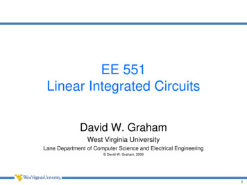
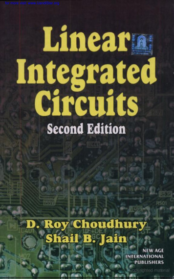
Last Updated: 2019-09-04 11:063If the setup is correct, you should see PRIMLIB, TECH XT018, and TECH XT018 HD under XFABLibs.These are the PDK-related libraries which will be extensively used later in the lab and also during the project.In Cadence there’s a relatively straightforward hierarchical organization structure. Libraries (leftmost column) are collections of Cells, and Cells are collections of Views.The first thing you’ll need is a new library. To do this, go to the library manager and click File New Library. A new window will pop up. Type ‘lab2’ in the name field an press OK.Figure 2: New Library windowAt this point, Cadence will prompt you for something called a Technology File (fair warning that Cadencelikes pop-unders). The technology file is a library or group of libraries that all cell views inside of your newlibrary will automatically reference. This basically means that you will not have to import models everytime you run a new simulation.Choose “Reference existing technology libraries” and add TECH XT018 and TECH XT018 HD by highlighting them on the left side and clicking the right-pointing arrow. Press OK when finished.UCB EE 140/240A, Fall 2019, Lab 2, All Rights Reserved. This may not be publicly shared without explicit permission.3
Last Updated: 2019-09-04 11:064Figure 3: Windows to choose technology files for your new libraryNow that you have a library, you can create your first schematic. Select your new lab2 library in the librarymanager, and click File New Cell View. When prompted, name the new cell view inverter andselect “schematic” from the drop-down menu and “schematic” should auto-fill under View. Click OK, andthe schematic editor should open up. Now we can build a virtual representation of our circuit at the transistorlevel.Figure 4: New Cell windowTo instantiate circuit elements in the schematic, press the ‘i’ key. This will bring up the Add Instancewindow and the Component Browser. To put an NMOS transistor, go to Component Browser, changeLibrary to PRIMLIB, and scroll down to ne. Checking the “Show Categories” box at the top left may aid inyour search. This selection should auto-fill in the Add Instance window. You can also type these referencesinto the fields manually. As soon as you do this, you will be prompted with lots of new options. What youare actually doing at this point is instantiating a parameterized cell, or P-cell for short. You can parameterizethe transistor gate width, length, and fingers. Your choices will be reflected in the schematic. For now,let’s stick with a minimum-sized transistor with a length of 180nm and a width of 220nm. Press the “hide”button or hit the Enter key in the Add Instance menu and click down the transistor into your schematic.Press Escape to stop adding components. If you ever want to change a p-cell’s properties after placing it inthe schematic, click on it and press ‘q’.UCB EE 140/240A, Fall 2019, Lab 2, All Rights Reserved. This may not be publicly shared without explicit permission.4
Last Updated: 2019-09-04 11:065Following those same instructions, instantiate a PMOS transistor (pe) with a 180nm length and 220nmwidth. Press the ‘w’ key to open up the “Add Wire” window. This will allow you to make connectionsbetween nodes. Simply click on the red squares (contacts) in the schematic view., and make connectionsneeded for an inverter circuit. Be sure to connect the bulk terminals of the NMOS and the PMOS to theirrespective sources (in this case ground and the supply, respectively).To navigate the schematic, use the arrow keys on the keyboard to pan around. You can zoom in/out byscrolling. You can zoom into a specific area by click-dragging a box with the right mouse button around theregion of interest. If the circuit ever disappears or you want to look at the whole circuit, press the ‘f’ key.The last thing you need is the pins to indicate the input, output, supply, and ground of your inverter. Thisway your cell view can interface with higher-level schematics (more on this later). Press ‘p’ to open up the“Add Pins” window, type the names of your pins (you can add more than one by separating their names withspaces). Place your pins in the schematic and wire them up.You should establish these pins:Pin NameVINVOUTVDDVSSPin TypeinputoutputinputOutputinputOutputFigure 5: Add Pin windowIf you followed the instructions, your schematic should look something like this:UCB EE 140/240A, Fall 2019, Lab 2, All Rights Reserved. This may not be publicly shared without explicit permission.5
Last Updated: 2019-09-04 11:066Figure 6: Inverter schematicWhen it does, press the “Check and Save” button (a box with a check mark). Leave the schematic editoropen for now; we’ll need it for the later portions of the lab.One more quick note: sometimes it helps to label nodes instead of directly connecting them with a wire. Toconnect two nodes, just label them with the same name! To create a label, press ‘l’ (that’s ell), type in thedesired node name, and click on the wire in the schematic.5Creating a Symbol ViewNow that your schematic is finished, we need to create a symbol for it. Click Create Cellview FromCellview. A pop to create a symbol appears. After you press OK, a new pop-up (or under) titled “SymbolGeneration Options” shows up. Set up your pin locations such that VSS is placed at the bottom, but you canotherwise leave things as they are.UCB EE 140/240A, Fall 2019, Lab 2, All Rights Reserved. This may not be publicly shared without explicit permission.6
Last Updated: 2019-09-04 11:067Figure 7: Options for creating a cellview from a cellviewAfter you press OK, you’ll have the opportunity to place any missing pins in the symbol editor. Note thatthe red dot is the actual point where a wire will connect, so put it toward the edge of your symbol. Drawvarious shapes using the shape buttons at the top make your symbol look like an actual inverter. Save yoursymbol view when finished.UCB EE 140/240A, Fall 2019, Lab 2, All Rights Reserved. This may not be publicly shared without explicit permission.7
Last Updated: 2019-09-04 11:0668Circuit Simulation with ADEBefore simulating anything, you’ll need to build a test bench for your inverter. To do this, create a schematiccalled zz inverter in your lab2 library. Placing “zz” at the start of each of your test benches allows youto quickly find any testbenches you’ve made since it will always place them at the bottom of the alphabetizedlist of cells.In your test bench schematic, instantiate a cell called vpulse from the analogLib library (under CadenceLibs).Set the following properties (Cadence will populate the correct units for you)ParameterDC VoltageVoltage 1Voltage 2PeriodRise timeFall timePulse widthValueVIN0120n10p10p10nNotice how we didn’t set the DC voltage to a numerical value! Instead, we assigned it to the variable “VIN”.Assigning parameters to variables allows you to change them easily and sweep them in the simulator.Now instantiate the inverter symbol you created earlier, and a vdc from the library analogLib. Set itsDC voltage to 1V.Connect all the circuit components together with wires. You should label the input and output nets to easilyidentify them (press ‘l’ (that’s ell)). Notice how we didn’t actually need to draw a wire for VDD—instead,we labeled both nets the same, and they’re now shorted together.UCB EE 140/240A, Fall 2019, Lab 2, All Rights Reserved. This may not be publicly shared without explicit permission.8
Last Updated: 2019-09-04 11:069Figure 8: Schematic of the testbenchClick “Check and Save”. You’ll get a few warnings and a couple blinking boxes (visible in Figure ?) whichyou can safely ignore.Now you can finally set up the simulation for your inverter. Click Launch ADE L to open up the legendaryVirtuoso Analog Design Environment (ADE). This tool is a little obtuse but extremely powerful. Let’s startwith two simple simulations: a DC simulation to determine our inverter’s voltage transfer characteristic, anda ransient simulation to determine its propagation delay.First let’s set up the design variables. Click on Variables Copy From Cellview. Remember how you setthe vpulse DC voltage to a variable? Here’s where you can use it in your simulation. Set the default valueof VIN to 1V (just type in 1 and Cadence will give you the right units).Click on Analyses Choose to open the analysis window. Select “dc”, set the sweep variable to “DesignVariable” and use “VIN” as the variable name. Sweep it from 0V to 1V with a step size of 10mV. ClickOK.UCB EE 140/240A, Fall 2019, Lab 2, All Rights Reserved. This may not be publicly shared without explicit permission.9
Last Updated: 2019-09-04 11:0610Figure 9: DC simulation setup. Note that you don’t need to Save DC Operating Point—it’s a useful debugging tool when designing larger circuits.Follow the same procedure to create a transient simulation with a duration of 100ns.UCB EE 140/240A, Fall 2019, Lab 2, All Rights Reserved. This may not be publicly shared without explicit permission.10
Last Updated: 2019-09-04 11:0611Figure 10: Transient simulation setupTo make the simulator automatically plot the desired waveforms, click Tools Calculator. We’ll want theDC sweep values for the input and output as well as the transient voltage values for the input and output. Toget the DC sweep voltage, click “vs” and then click “OUT” on your schematic. Do NOT close this window.Figure 11: Partial capture of the calculator window with “vs” selected.In your ADE window, right click the “Outputs” region and select Edit. Press “Get Expression”, and theexpression from the calculator will appear in the “Expression” box. Name it “dcs vout” and press “Add”.This will add your expression to your outputs.UCB EE 140/240A, Fall 2019, Lab 2, All Rights Reserved. This may not be publicly shared without explicit permission.11
Last Updated: 2019-09-04 11:0612Figure 12: Windows for adding your calculator expression to your outputRepeat this for “dcs vin”. The process for adding the transient voltage is similar, but instead of selecting“vs”, choose “vt”. Your ADE window should now look something like this:UCB EE 140/240A, Fall 2019, Lab 2, All Rights Reserved. This may not be publicly shared without explicit permission.12
Last Updated: 2019-09-04 11:0613Figure 13: ADE window after adding all the outputsTo run the simulation, click the green “play” icon on the right side of your ADE window. Close the “What’sNew” poop-up and the simulation will run. The input and output waveforms should be plotted automatically.Figure 14: Automatically plotted input and output waveformsFrom the DC sweep, find the gain by estimating the slope of the curve where the output is roughly 0.5Vusing markers (pressing “h” for horizontal markers and “v” for vertical markers). Need to fix hotkeysAnother option is to use the calculator again. Using the “wave” selection option, click the DC responseon your graph. To calculate the derivative, use the expression you get as the argument for the functionderiv(). You can plot the result in a new window and evaluate the gain from there. Inverters are normallyUCB EE 140/240A, Fall 2019, Lab 2, All Rights Reserved. This may not be publicly shared without explicit permission.13
Last Updated: 2019-09-04 11:0614associated with digital circuits, but they can be used as amplifiers as well.Figure 15: Plotting the derivative of the output voltage with respect to the x-axis (the variable VIN)If your plot doesn’t seem very smooth, try shrinking the step size in your DC sweep.Using these two methods, record the DC gain for the lab report.The propagation delay of the inverter is defined as the time between the input crossing VDD2 and the outputVDDtransitioning to 2 . Use the cursors on the transient simulation to measure the high-to-low and low-to-highpropagation delays. Provide a plot and record these values for the lab report.Before closing the ADE window, you can save a runset state file for your future usage. To do this, click onthe save button in ADE window. Choose Cellview for the Save State Option option, and click onOK to save it.UCB EE 140/240A, Fall 2019, Lab 2, All Rights Reserved. This may not be publicly shared without explicit permission.14
Last Updated: 2019-09-04 11:0615Figure 16: Save runset state7Creating a Layout ViewIn your schematic view for your inverter, click Launch Layout XL. Choose “Create New” with theAutomatic configuration. This will open the Layout XL Editor in a new window. Press “e” to open up theDisplay Options window. You’ll want to make sure the X and Y Snap Spacing are set to 0.005 (5nm). UnderDisplay Levels, set “Stop” to 32.UCB EE 140/240A, Fall 2019, Lab 2, All Rights Reserved. This may not be publicly shared without explicit permission.15
Last Updated: 2019-09-04 11:0616Figure 17: The Display Options windowBecause you opened Layout XL from your schematic view, there is a box at the bottom left to “Generate AllFrom Source” . Clicking on this will open up the following windowUCB EE 140/240A, Fall 2019, Lab 2, All Rights Reserved. This may not be publicly shared without explicit permission.16
Last Updated: 2019-09-04 11:0617Figure 18: The Generate Layout window.Uncheck “I/O Pins” and “PR Boundary”, then press OK. This will automatically populate your layout withall the necessary cells for your layout with all the correct properties. If you want to change the propertiesof any of these cells at any point, click on the cell and press ‘q’ to open up the properties window. You’llalso notice that clicking on nets and devices in the schematic will highlight in both the schematic and thelayout—this is really helpful for routing!Figure 19: Clicking on the VOUT net highlights the net in both the schematic and the layout (the latter isboxed in white)Now we’ll make metal lines for the power supply. To specify the material, go to the “Layers” toolbox onUCB EE 140/240A, Fall 2019, Lab 2, All Rights Reserved. This may not be publicly shared without explicit permission.17
Last Updated: 2019-09-04 11:0618Figure 20: The Layers toolbar with MET1 highlighted and selectedthe left side. Find MET1 whose purpose is drw.Now press the ‘p’ key to create a path. If you want to change the thickness of the path, press “F3” and makethe changes as you like. Now draw the paths so they form stripes above and below your MOSFETs. Doubleclick to end the path. Don’t worry if they’re not perfectly aligned to anything for now, you can alwayschange what you’ve drawn later. Change the thickness of your path to 0.6.If you’d like to change any properties of your drawn boxes or cells, click on the item of interest and press‘q’.Now using MET1, wire up the sources and drains of your devices to the appropriate routings. Just lookingat MET1, your routing should look something like thisUCB EE 140/240A, Fall 2019, Lab 2, All Rights Reserved. This may not be publicly shared without explicit permission.18
Last Updated: 2019-09-04 11:0619Figure 21: An example of MET1 routing for the inverterYou’ve connected the sources and drains of the devices now. At this point we haven’t connected the gates,but it’s important we don’t forget the body contact of the device as well. Press ‘o’ (that’s oh) and a newwindow to create vias will appear. In the “Via Definition” drop-down, choose ND C, and in the radio dialsat the top choose “Shape(s)” in the “Compute From” selection. Click on the power rail meant for VDD atthe top and a via will automatically be put down to contact the body.Repeat the same process for VSS, but with PD C instead.UCB EE 140/240A, Fall 2019, Lab 2, All Rights Reserved. This may not be publicly shared without explicit permission.19
Last Updated: 2019-09-04 11:0620Figure 22: The Create Via window for connecting the VDD power rail to the device bodyAll we have left to connect are the gates of our transistors. Connect the gates of your transistors with layerPOLY1 using ‘p’ again.UCB EE 140/240A, Fall 2019, Lab 2, All Rights Reserved. This may not be publicly shared without explicit permission.20
Last Updated: 2019-09-04 11:0621Figure 23: POLY1 routing (green) with the active layer (DIFF, in red) and MET1 shown for clarityYou’ll notice that around the PMOS there’s a box in layer PIMP for P-Implant, and around the NMOSthere’s a box in layer NIMP for N-Implant. In an NMOS, the bulk is the substrate—implicitly shown inblack. A PMOS must be placed in an N-well to operate properly. THe N-well is automatically placed withthe PMOS, but too small to make connections. To draw a bigger N-well, find the NWELL drawing layer andpress ‘r’ to draw a rectangle that includes the PMOS and the top metal line.UCB EE 140/240A, Fall 2019, Lab 2, All Rights Reserved. This may not be publicly shared without explicit permission.21
Last Updated: 2019-09-04 11:0622Figure 24: The layout so far (yours does not need to look exactly like this, just be sure the yellow boxNWELL encompasses the top rail and the PMOS device)8Design Rule Checking (DRC)The DRC checker verifies that your drawn layers obey all of the design rules. These design rules are providedby the IC foundry to ensure that the IC devices perform to specification. The design rules document can befound at LOCATION ON BCOURSES.To run DRC, go to the menu bar and click Assura Run DRC. Make sure the library, cell, and the vieware set to lab2, inverter, and layout. In the third section, change the Rule Set to “DRC % Dummy Output”.Click “Set Switches” and click “noAntenna”. This turns off any antenna DRC checks—this is typically runat the top-level for a full chip.UCB EE 140/240A, Fall 2019, Lab 2, All Rights Reserved. This may not be publicly shared without explicit permission.22
Last Updated: 2019-09-04 11:0623Figure 25: The DRC options windowPress OK. A few other windows may show up asking about overwriting any AssuraDRC files—press OK onthese too. You’ll be prompted asking if you’d like to see the DRC results—click OK. If you have no DRCerrors, a Virtuoso window should appear saying so. Otherwise, another window will appear with the errorsdescribed. The errors may be difficult to understand. Try to decode what needs to be fixed (usually this willhave to do with the spacing or overlap between components and paths). Ask your GSI if you’re stuck.9Adding Pins to the Layout ViewRemember that, in the schematic and symbol, we had pins for the input and output of the inverter. PressCreate Pin and (another) pop-up will show upUCB EE 140/240A, Fall 2019, Lab 2, All Rights Reserved. This may not be publicly shared without explicit permission.23
Last Updated: 2019-09-04 11:0624Figure 26: Create Pin window. Select the window and the I/O type to match your schematicType in your terminal name and change the I/O type to match your schematic (e.g. inputOutput, input, etc.).Click and draw a rectangle where you’d like to place the pin. Where you’ve drawn it, select the pin, press‘q’, and change the layer to MET1 pin. Make sure that you have a connection from POLY1 to MET1 at thegate, otherwise your pin will not be physically connected to your device!For clarity, it helps to add labels to your pins so you know what they are. Press Create Label. Separatedifferent labels with a space.UCB EE 140/240A, Fall 2019, Lab 2, All Rights Reserved. This may not be publicly shared without explicit permission.24
Last Updated: 2019-09-04 11:0625Figure 27: Create Label window. You can change the height of your letters as well as the font.10Layout Versus Schematic (LVS) VerificationNow, we need to check to see whether the transistors and pins we placed here actually match up with thetransistors we placed in schematic. To do this, we run a layout vs. schematic (LVS) checker. From yourLayout window, press Assura Run LVS. Your “Run Assura LVS” menu should look like this:UCB EE 140/240A, Fall 2019, Lab 2, All Rights Reserved. This may not be publicly shared without explicit permission.25
Last Updated: 2019-09-04 11:0626Figure 28: LVS windowPress OK to run LVS. If your layout matches your schematic, you will see the following message:UCB EE 140/240A, Fall 2019, Lab 2, All Rights Reserved. This may not be publicly shared without explicit permission.26
Last Updated: 2019-09-04 11:0627Figure 29: No LVS errors!If you have any LVS errors, correct them by making the appropriate adjustments to your layout. Rememberto run DRC check again afterward to make sure your update doesn’t violate any design rules. If you see a lotof pin mismatch errors over pins which you think are correct, make sure the type out pin (e.g. inputOutput,input, output, etc.) is correct.At this point, your layout now passes DRC and LVS âĂŞ a huge milestone in the IC design process. Next,we will examine how the physical placement of transistors (layout) impacts circuit performance.11Parasitic ExtractionStart QRC in your layout window by clicking on Quantus Run Assura - Quantus QRC, and the followingwindow will pop up.Figure 30: QRC start window.Click on OK and you will see QRC setting window. In the Setup tab, make sure that RuleSet isdefault and Output is Extracted View.UCB EE 140/240A, Fall 2019, Lab 2, All Rights Reserved. This may not be publicly shared without explicit permission.27
Last Updated: 2019-09-04 11:0628Figure 31: QRC Setup tap.In Extraction tab, make Extraction Type as RC, Cap Coupling Mode as Coupled andRef Node as your circuit ground node (VSS in this lab). For other tabs, just use its default settingsfor now.UCB EE 140/240A, Fall 2019, Lab 2, All Rights Reserved. This may not be publicly shared without explicit permission.28
Last Updated: 2019-09-04 11:0629Figure 32: QRC Extraction tap.Click on OK and you will get a window showing QRC is running.UCB EE 140/240A, Fall 2019, Lab 2, All Rights Reserved. This may not be publicly shared without explicit permission.29
Last Updated: 2019-09-04 11:0630Figure 33: QRC running window.If QRC is done successfully, the following window will pop up.Figure 34: QRC running successfully.However, If QRC failed, you will get the following window. You need to click on Yes and read the log fileto get the problems.Figure 35: QRC failed.After finish this step. You will get analog extracted view in your inverter views.UCB EE 140/240A, Fall 2019, Lab 2, All Rights Reserved. This may not be publicly shared without explicit permission.30
Last Updated: 2019-09-04 11:0631Figure 36: Extraction view.12Parasitic Extracted Circuit SimulationTo run post-layout simulation, you need to create another cellview in your zz inverter testbench.In Library Manager, click File New Cell View and choose config in Type and click OK. TheVirtuoso Hierarchy Editor and New Configuration window will pop up. In the “New Configuration” window choose Schematic for “View”. Click on Use Template button at the bottom, andchoose spectre for Name in the pop-up Use Template window.UCB EE 140/240A, Fall 2019, Lab 2, All Rights Reserved. This may not be publicly shared without explicit permission.31
Last Updated: 2019-09-04 11:0632Figure 37: Virtuoso Hierarchy Editor and New Configuration window.Click on OK and the Global Bindings part will be automatically filled.Figure 38: New Configuration window after filled.UCB EE 140/240A, Fall 2019, Lab 2, All Rights Reserved. This may not be publicly shared without explicit permission.32
Last Updated: 2019-09-04 11:0633Click OK and in the Virtuoso Hierarchy Window, all the cells used in your testbench will be listed in theCell Bindings tab like following.Figure 39: Hierarchy Editor window.Right click on your top DUT (design under test) cell (inverter in this lab), and choose the analog extractedview. Save this view, and your Hierarchy Editor window will be like this:UCB EE 140/240A, Fall 2019, Lab 2, All Rights Reserved. This may not be publicly shared without explicit permission.33
Last Updated: 2019-09-04 11:0634Figure 40: Hierarchy Editor window after choose the post-layoout view.Click on the Open button in the Top Cell part. The testbench will open again, but with a Config view(You can also open it within Library Manager).UCB EE 140/240A, Fall 2019, Lab 2, All Rights Reserved. This may not be publicly shared without explicit permission.34
Last Updated: 2019-09-04 11:0635Figure 41: Open config view.For now, you can just close the Hierarchy Editor window. In the testbench, you can double check you areusing the post-layout netlist by decending into the inverter. The first entry should be analog extracted,and if you go into the netlist, you will see the back-annotations transistors, resistors and capacitors in thelayout (If you cannot see it, use Shift F to swap the display level).Figure 42: Decend into extracted view.Check and save your schematic and launch "ADE L" again. Load the runset you saved in the previoussimulation.UCB EE 140/240A, Fall 2019, Lab 2, All Rights Reserved. This may not be publicly shared without explicit permission.35
Last Updated: 2019-09-04 11:0636Figure 43: Load runset.The ADE window will be like the this:Figure 44: ADE window after load the runset.Click Simulation Netlist Create. The netlist should be simulated with all the parasitics included. Lookat the parasitics to get a feel for their values. Save a copy of the netlist (either text or screenshot) toinclude in your lab report. Re-run the simulation, the results window will pop up and this is your postlayout simulation results. You can compare it with the schematic simulation results. Record the DC gainand propagation delay again.UCB EE 140/240A, Fall 2019, Lab 2, All Rights Reserved. This may not be publicly shared without explicit permission.36
Last Updated: 2019-09-04 11:0637Figure 45: Post-layout simulation results.13Deliverables(1) Schematic simulationa. DC gainb. High-low propagation delayc. Low-high propagation delay(2) Screenshot of finished inverter layout(3) Netlist with extracted parasitics(4) Extracted simulationa. DC gainb. High-low propagation delayc. Low-high propagation delayUCB EE 140/240A, Fall 2019, Lab 2, All Rights Reserved. This may not be publicly shared without explicit permission.37
Sep 04, 2019 · Last Updated: 2019-09-04 11:06 3 If the setup is correct, you should see PRIMLIB, TECH_XT018, and TECH_XT018_HD under XFABLibs. These are the PDK-related libraries which will be exten