Transcription
Lent Term, 2015ElectromagnetismUniversity of Cambridge Part IB Mathematical TriposDavid TongDepartment of Applied Mathematics and Theoretical Physics,Centre for Mathematical Sciences,Wilberforce Road,Cambridge, CB3 OBA, ng@damtp.cam.ac.uk
Maxwell Equations ·E ρ 0 ·B 0 E B t E B µ0 J 0 t–1–
Recommended Books and ResourcesThere is more or less a well established route to teaching electromagnetism. A numberof good books follow this. David J. Griffiths, “Introduction to Electrodynamics”A superb book. The explanations are clear and simple. It doesn’t cover quite as muchas we’ll need for these lectures, but if you’re looking for a book to cover the basics thenthis is the first one to look at. Edward M. Purcell and David J. Morin “Electricity and Magnetism”Another excellent book to start with. It has somewhat more detail in places thanGriffiths, but the beginning of the book explains both electromagnetism and vectorcalculus in an intertwined fashion. If you need some help with vector calculus basics,this would be a good place to turn. If not, you’ll need to spend some time disentanglingthe two topics. J. David Jackson, “Classical Electrodynamics”The most canonical of physics textbooks. This is probably the one book you can findon every professional physicist’s shelf, whether string theorist or biophysicist. It willsee you through this course and next year’s course. The problems are famously hard.But it does have div, grad and curl in polar coordinates on the inside cover. A. Zangwill, “Modern Electrodynamics”A great book. It is essentially a more modern and more friendly version of Jackson. Feynman, Leighton and Sands, “The Feynman Lectures on Physics, Volume II”Feynman’s famous lectures on physics are something of a mixed bag. Some explanationsare wonderfully original, but others can be a little too slick to be helpful. And much ofthe material comes across as old-fashioned. Volume two covers electromagnetism and,in my opinion, is the best of the three.A number of excellent lecture notes, including the Feynman lectures, are availableon the web. Links can be found on the course ml–2–
Contents1. Introduction1.1 Charge and Current1.1.1 The Conservation Law1.2 Forces and Fields1.2.1 The Maxwell Equations124462. Electrostatics2.1 Gauss’ Law2.1.1 The Coulomb Force2.1.2 A Uniform Sphere2.1.3 Line Charges2.1.4 Surface Charges and Discontinuities2.2 The Electrostatic Potential2.2.1 The Point Charge2.2.2 The Dipole2.2.3 General Charge Distributions2.2.4 Field Lines2.2.5 Electrostatic Equilibrium2.3 Electrostatic Energy2.3.1 The Energy of a Point Particle2.3.2 The Force Between Electric Dipoles2.4 Conductors2.4.1 Capacitors2.4.2 Boundary Value Problems2.4.3 Method of Images2.4.4 Many many more problems2.4.5 A History of 7393. Magnetostatics3.1 Ampère’s Law3.1.1 A Long Straight Wire3.1.2 Surface Currents and Discontinuities3.2 The Vector Potential3.2.1 Magnetic Monopoles414242434647–3–
3.33.43.53.2.2 Gauge Transformations3.2.3 Biot-Savart Law3.2.4 A Mathematical Diversion: The Linking NumberMagnetic Dipoles3.3.1 A Current Loop3.3.2 General Current DistributionsMagnetic Forces3.4.1 Force Between Currents3.4.2 Force and Energy for a Dipole3.4.3 So What is a Magnet?Units of Electromagnetism3.5.1 A History of Magnetostatics4849525454565757596264654. Electrodynamics4.1 Faraday’s Law of Induction4.1.1 Faraday’s Law for Moving Wires4.1.2 Inductance and Magnetostatic Energy4.1.3 Resistance4.1.4 Michael Faraday (1791-1867)4.2 One Last Thing: The Displacement Current4.2.1 Why Ampère’s Law is Not Enough4.3 And There Was Light4.3.1 Solving the Wave Equation4.3.2 Polarisation4.3.3 An Application: Reflection off a Conductor4.3.4 James Clerk Maxwell (1831-1879)4.4 Transport of Energy: The Poynting Vector4.4.1 The Continuity Equation Revisited6767697174777980828487899192945. Electromagnetism and Relativity5.1 A Review of Special Relativity5.1.1 Four-Vectors5.1.2 Proper Time5.1.3 Indices Up, Indices Down5.1.4 Vectors, Covectors and Tensors5.2 Conserved Currents5.2.1 Magnetism and Relativity5.3 Gauge Potentials and the Electromagnetic Tensor959596979899102103105–4–
5.45.55.3.1 Gauge Invariance and Relativity5.3.2 The Electromagnetic Tensor5.3.3 An Example: A Boosted Line Charge5.3.4 Another Example: A Boosted Point Charge5.3.5 Lorentz ScalarsMaxwell Equations5.4.1 The Lorentz Force Law5.4.2 Motion in Constant FieldsEpilogue–5–105106109110111113115117118
AcknowledgementsThese lecture notes contain material covering two courses on Electromagnetism.In Cambridge, these courses are called Part IB Electromagnetism and Part II Electrodynamics. The notes owe a debt to the previous lecturers of these courses, includingNatasha Berloff, John Papaloizou and especially Anthony Challinor.The notes assume a familiarity with Newtonian mechanics and special relativity, ascovered in the Dynamics and Relativity notes. They also assume a knowledge of vectorcalculus. The notes do not cover the classical field theory (Lagrangian and Hamiltonian)section of the Part II course.–6–
1. IntroductionThere are, to the best of our knowledge, four forces at play in the Universe. At the verylargest scales — those of planets or stars or galaxies — the force of gravity dominates.At the very smallest distances, the two nuclear forces hold sway. For everything inbetween, it is force of electromagnetism that rules.At the atomic scale, electromagnetism (admittedly in conjunction with some basicquantum effects) governs the interactions between atoms and molecules. It is the forcethat underlies the periodic table of elements, giving rise to all of chemistry and, throughthis, much of biology. It is the force which binds atoms together into solids and liquids.And it is the force which is responsible for the incredible range of properties thatdifferent materials exhibit.At the macroscopic scale, electromagnetism manifests itself in the familiar phenomena that give the force its name. In the case of electricity, this means everything fromrubbing a balloon on your head and sticking it on the wall, through to the fact that youcan plug any appliance into the wall and be pretty confident that it will work. For magnetism, this means everything from the shopping list stuck to your fridge door, throughto trains in Japan which levitate above the rail. Harnessing these powers through theinvention of the electric dynamo and motor has transformed the planet and our liveson it.As if this wasn’t enough, there is much more to the force of electromagnetism for itis, quite literally, responsible for everything you’ve ever seen. It is the force that givesrise to light itself.Rather remarkably, a full description of the force of electromagnetism is contained infour simple and elegant equations. These are known as the Maxwell equations. Thereare few places in physics, or indeed in any other subject, where such a richly diverseset of phenomena flows from so little. The purpose of this course is to introduce theMaxwell equations and to extract some of the many stories they contain.However, there is also a second theme that runs through this course. The force ofelectromagnetism turns out to be a blueprint for all the other forces. There are variousmathematical symmetries and structures lurking within the Maxwell equations, structures which Nature then repeats in other contexts. Understanding the mathematicalbeauty of the equations will allow us to see some of the principles that underly the lawsof physics, laying the groundwork for future study of the other forces.–1–
1.1 Charge and CurrentEach particle in the Universe carries with it a number of properties. These determinehow the particle interacts with each of the four forces. For the force of gravity, thisproperty is mass. For the force of electromagnetism, the property is called electriccharge.For the purposes of this course, we can think of electric charge as a real number,q R. Importantly, charge can be positive or negative. It can also be zero, in whichcase the particle is unaffected by the force of electromagnetism.The SI unit of charge is the Coulomb, denoted by C. It is, like all SI units, a parochialmeasure, convenient for human activity rather than informed by the underlying lawsof the physics. (We’ll learn more about how the Coulomb is defined in Section 3.5).At a fundamental level, Nature provides us with a better unit of charge. This followsfrom the fact that charge is quantised: the charge of any particle is an integer multipleof the charge carried by the electron which we denoted as e, withe 1.60217657 10 19 CA much more natural unit would be to simply count charge as q ne with n Z.Then electrons have charge 1 while protons have charge 1 and neutrons have charge0. Nonetheless, in this course, we will bow to convention and stick with SI units.(An aside: the charge of quarks is actually q e/3 and q 2e/3. This doesn’tchange the spirit of the above discussion since we could just change the basic unit. But,apart from in extreme circumstances, quarks are confined inside protons and neutronsso we rarely have to worry about this).One of the key goals of this course is to move beyond the dynamics of point particlesand onto the dynamics of continuous objects known as fields. To aid in this, it’s usefulto consider the charge density,ρ(x, t)defined as charge per unit volume. The total charge Q in a given region V is simplyRQ V d3 x ρ(x, t). In most situations, we will consider smooth charge densities, whichcan be thought of as arising from averaging over many point-like particles. But, onoccasion, we will return to the idea of a single particle of charge q, moving on sometrajectory r(t), by writing ρ qδ(x r(t)) where the delta-function ensures that allthe charge sits at a point.–2–
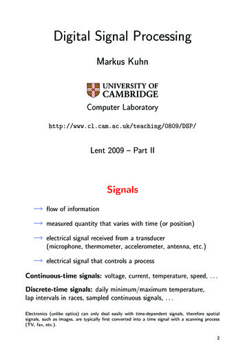
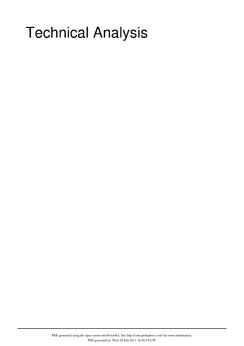
More generally, we will need to describe the movement of charge from one place toanother. This is captured by a quantity known as the current density J(x, t), definedas follows: for every surface S, the integralZJ · dSI Scounts the charge per unit time passing through S. (Here dS is the unit normal toS). The quantity I is called the current. In this sense, the current density is thecurrent-per-unit-area.The above is a rather indirect definition of the current density. To get a more intuitive picture, consider acontinuous charge distribution in which the velocity of asmall volume, at point x, is given by v(x, t). Then, neglecting relativistic effects, the current density isSJ ρvIn particular, if a single particle is moving with velocityFigure 1: Current fluxv ṙ(t), the current density will be J qvδ 3 (x r(t)).This is illustrated in the figure, where the underlying charged particles are shown asred balls, moving through the blue surface S.As a simple example, consider electrons moving along a wire. We model the wire as a longAcylinder of cross-sectional area A as shown below. The electrons move with velocity v, parallel to the axis of the wire. (In reality, the elecvtrons will have some distribution of speeds; weFigure 2: The wiretake v to be their average velocity). If there aren electrons per unit volume, each with chargeq, then the charge density is ρ nq and the current density is J nqv. The currentitself is I J A.Throughout this course, the current density J plays a much more prominent rolethan the current I. For this reason, we will often refer to J simply as the “current”although we’ll be more careful with the terminology when there is any possibility forconfusion.–3–
1.1.1 The Conservation LawThe most important property of electric charge is that it’s conserved. This, of course,means that the total charge in a system can’t change. But it means much more thanthat because electric charge is conserved locally. An electric charge can’t just vanishfrom one part of the Universe and turn up somewhere else. It can only leave one pointin space by moving to a neighbouring point.The property of local conservation means that ρ can change in time only if thereis a compensating current flowing into or out of that region. We express this in thecontinuity equation, ρ ·J 0 t(1.1)This is an important equation. It arises in any situation where there is some quantitythat is locally conserved.To see why the continuity equation captures the right physics, it’s best to considerthe change in the total charge Q contained in some region V .ZZZdQ ρ33 dx d x · J J · dSdt tVVSRFrom our previous discussion, S J · dS is the total current flowing out through theboundary S of the region V . (It is the total charge flowing out, rather than in, becausedS is the outward normal to the region V ). The minus sign is there to ensure that ifthe net flow of current is outwards, then the total charge decreases.If there is no current flowing out of the region, then dQ/dt 0. This is the statementof (global) conservation of charge. In many applications we will take V to be all ofspace, R3 , with both charges and currents localised in some compact region. Thisensures that the total charge remains constant.1.2 Forces and FieldsAny particle that carries electric charge experiences the force of electromagnetism. Butthe force does not act directly between particles. Instead, Nature chose to introduceintermediaries. These are fields.In physics, a “field” is a dynamical quantity which takes a value at every point inspace and time. To describe the force of electromagnetism, we need to introduce two–4–
fields, each of which is a three-dimensional vector. They are called the electric field Eand the magnetic field B,E(x, t) and B(x, t)When we talk about a “force” in modern physics, we really mean an intricate interplaybetween particles and fields. There are two aspects to this. First, the charged particlescreate both electric and magnetic fields. Second, the electric and magnetic fields guidethe charged particles, telling them how to move. This motion, in turn, changes thefields that the particles create. We’re left with a beautiful dance with the particles andfields as two partners, each dictating the moves of the other.This dance between particles and fields provides a paradigm which all other forces inNature follow. It feels like there should be a deep reason that Nature chose to introducefields associated to all the forces. And, indeed, this approach does provide one overriding advantage: all interactions are local. Any object — whether particle or field —affects things only in its immediate neighbourhood. This influence can then propagatethrough the field to reach another point in space, but it does not do so instantaneously.It takes time for a particle in one part of space to influence a particle elsewhere. Thislack of instantaneous interaction allows us to introduce forces which are compatiblewith the theory of special relativity, something that we will explore in more detail inSection 5The purpose of this course is to provide a mathematical description of the interplaybetween particles and electromagnetic fields. In fact, you’ve already met one side ofthis dance: the position r(t) of a particle of charge q is dictated by the electric andmagnetic fields through the Lorentz force law,F q(E ṙ B)(1.2)The motion of the particle can then be determined through Newton’s equation F mr̈.We explored various solutions to this in the Dynamics and Relativity course. Roughlyspeaking, an electric field accelerates a particle in the direction E, while a magneticfield causes a particle to move in circles in the plane perpendicular to B.We can also write the Lorentz force law in terms of the charge distribution ρ(x, t)and the current density J(x, t). Now we talk in terms of the force density f (x, t), whichis the force acting on a small volume at point x. Now the Lorentz force law readsf ρE J B–5–(1.3)
1.2.1 The Maxwell EquationsIn this course, most of our attention will focus on the other side of the dance: the wayin which electric and magnetic fields are created by charged particles. This is describedby a set of four equations, known collectively as the Maxwell equations. They are:ρ 0(1.4) ·B 0(1.5) ·E E B 0 t B µ0 0 E µ0 J t(1.6)(1.7)The equations involve two constants. The first is the electric constant (known also, inslightly old-fashioned terminology, as the permittivity of free space), 0 8.85 10 12 m 3 Kg 1 s2 C 2It can be thought of as characterising the strength of the electric interactions. Theother is the magnetic constant (or permeability of free space),µ0 4π 10 7 m Kg C 2 1.25 10 6 m Kg C 2The presence of 4π in this formula isn’t telling us anything deep about Nature. It’smore a reflection of the definition of the Coulomb as the unit of charge. (We will explainthis in more detail in Section 3.5). Nonetheless, this can be thought of as characterisingthe strength of magnetic interactions (in units of Coulombs).The Maxwell equations (1.4), (1.5), (1.6) and (1.7) will occupy us for the rest of thecourse. Rather than trying to understand all the equations at once, we’ll proceed bitby bit, looking at situations where only some of the equations are important. By theend of the lectures, we will understand the physics captured by each of these equationsand how they fit together.–6–
However, equally importantly, we will also explore the mathematical structure of theMaxwell equations. At first glance, they look just like four random equations fromvector calculus. Yet this couldn’t be further from the truth. The Maxwell equationsare special and, when viewed in the right way, are the essentially unique equationsthat can describe the force of electromagnetism. The full story of why these are theunique equations involves both quantum mechanics and relativity and will only be toldin later courses. But we will start that journey here. The goal is that by the end ofthese lectures you will be convinced of the importance of the Maxwell equations onboth experimental and aesthetic grounds.–7–
2. ElectrostaticsIn this section, we will be interested in electric charges at rest. This means that thereexists a frame of reference in which there are no currents; only stationary charges. Ofcourse, there will be forces between these charges but we will assume that the chargesare pinned in place and cannot move. The question that we want to answer is: whatis the electric field generated by these charges?Since nothing moves, we are looking for time independent solutions to Maxwell’sequations with J 0. This means that we can consistently set B 0 and we’re leftwith two of Maxwell’s equations to solve. They areρ 0(2.1) E 0(2.2) ·E andIf you fix the charge distribution ρ, equations (2.1) and (2.2) have a unique solution.Our goal in this section is to find it.2.1 Gauss’ LawBefore we proceed, let’s first present equation (2.1) in a slightly different form thatwill shed some light on its meaning. Consider some closed region V R3 of space.We’ll denote the boundary of V by S V . We now integrate both sides of (2.1) overV . Since the left-hand side is a total derivative, we can use the divergence theorem toconvert this to an integral over the surface S. We haveZZZ13d x ·E E · dS d3 x ρ 0 VVSThe integral of the charge density over V is simply the total charge contained in theRregion. We’ll call it Q d3 x ρ. Meanwhile, the integral of the electric field over S iscalled the flux through S. We learn that the two are related byZQE · dS (2.3) 0SThis is Gauss’s law. However, because the two are entirely equivalent, we also refer tothe original (2.1) as Gauss’s law.–8–
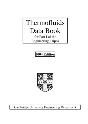
SS’SFigure 3: The flux through S and S 0 isthe same.Figure 4: The flux through S vanishes.Notice that it doesn’t matter what shape the surface S takes. As long as it surroundsa total charge Q, the flux through the surface will always be Q/ 0 . This is shown, forexample, in the left-hand figure above. A fancy way of saying this is that the integral ofthe flux doesn’t depend on the geometry of the surface, but does depend on its topologysince it must surround the charge Q. The choice of S is called the Gaussian surface;often there’s a smart choice that makes a particular problem simple.Only charges that lie inside V contribute to the flux. Any charges that lie outside willproduce an electric field that penetrates through S at some point, giving negative flux,but leaves through the other side of S, depositing positive flux. The total contributionfrom these charges that lie outside of V is zero, as illustrated in the right-hand figureabove.For a general charge distribution, we’ll need to use both Gauss’ law (2.1) and theextra equation (2.2). However, for rather special charge distributions – typically thosewith lots of symmetry – it turns out to be sufficient to solve the integral form of Gauss’law (2.3) alone, with the symmetry ensuring that (2.2) is automatically satisfied. Westart by describing these rather simple solutions. We’ll then return to the general casein Section 2.2.2.1.1 The Coulomb ForceWe’ll start by showing that Gauss’ law (2.3) reproduces the more familiar Coulombforce law that we all know and love. To do this, take a spherically symmetric chargedistribution, centered at the origin, contained within some radius R. This will be ourmodel for a particle. We won’t need to make any assumption about the nature of thedistribution other than its symmetry and the fact that the total charge is Q.–9–
We want to know the electric field at some radius r R. We take our Gaussian surface S to be a sphere of radiusr as shown in the figure. Gauss’ law statesZQE · dS 0SAt this point we make use of the spherical symmetry of theproblem. This tells us that the electric field must point radially outwards: E(x) E(r)r̂. And, since the integral isonly over the angular coordinates of the sphere, we can pullthe function E(r) outside. We haveZZQE · dS E(r) r̂ · dS E(r) 4πr2 0SSSRrFigure 5:where the factor of 4πr2 has arisen simply because it’s the area of the Gaussian sphere.We learn that the electric field outside a spherically symmetric distribution of chargeQ isE(x) Qr̂4π 0 r2(2.4)That’s nice. This is the familiar result that we’ve seen before. (See, for example, thenotes on Dynamics and Relativity). The Lorentz force law (1.2) then tells us that atest charge q moving in the region r R experiences a forceF Qqr̂4π 0 r2This, of course, is the Coulomb force between two static charged particles. Notice that,as promised, 1/ 0 characterises the strength of the force. If the two charges have thesame sign, so that Qq 0, the force is repulsive, pushing the test charge away fromthe origin. If the charges have opposite signs, Qq 0, the force is attractive, pointingtowards the origin. We see that Gauss’s law (2.1) reproduces this simple result that weknow about charges.Finally, note that the assumption of symmetry was crucial in our above analysis.Without it, the electric field E(x) would have depended on the angular coordinates ofthe sphere S and so been stuck inside the integral. In situations without symmetry,Gauss’ law alone is not enough to determine the electric field and we need to also use E 0. We’ll see how to do this in Section 2.2. If you’re worried, however, it’ssimple to check that our final expression for the electric field (2.4) does indeed solve E 0.– 10 –
Coulomb vs NewtonThe inverse-square form of the force is common to both electrostatics and gravity. It’sworth comparing the relative strengths of the two forces. For example, we can lookat the relative strengths of Newtonian attraction and Coulomb repulsion between twoelectrons. These are point particles with mass me and charge e given bye 1.6 10 19 Coulombsandme 9.1 10 31 KgRegardless of the separation, we haveFCoulombe21 FNewton4π 0 Gm2eThe strength of gravity is determined by Newton’s constant G 6.7 10 11 m3 Kg 1 s2 .Plugging in the numbers reveals something extraordinary:FCoulomb 1042FNewtonGravity is puny. Electromagnetism rules. In fact you knew this already. The mere actof lifting up you arm is pitching a few electrical impulses up against the gravitationalmight of the entire Earth. Yet the electrical impulses win.However, gravity has a trick up its sleeve. While electric charges come with bothpositive and negative signs, mass is only positive. It means that by the time we get tomacroscopically large objects — stars, planets, cats — the mass accumulates while thecharges cancel to good approximation. This compensates the factor of 10 42 suppressionuntil, at large distance scales, gravity wins after all.The fact that the force of gravity is so ridiculously tiny at the level of fundamentalparticles has consequence. It means that we can neglect gravity whenever we talkabout the very small. (And indeed, we shall neglect gravity for the rest of this course).However, it also means that if we would like to understand gravity better on these verytiny distances – for example, to develop a quantum theory of gravity — then it’s goingto be tricky to get much guidance from experiment.2.1.2 A Uniform SphereThe electric field outside a spherically symmetric charge distribution is always given by(2.4). What about inside? This depends on the distribution in question. The simplestis a sphere of radius R with uniform charge distribution ρ. The total charge isQ 4π 3R ρ3– 11 –
Let’s pick our Gaussian surface to be a sphere, centered atthe origin, of radius r R. The charge contained withinthis sphere is 4πρr3 /3 Qr3 /R3 , so Gauss’ law givesZQr3E · dS 0 R3SSrRAgain, using the symmetry argument we can write E(r) E(r)r̂ and computeZZQr3E · dS E(r) r̂ · dS E(r) 4πr2 0 R3SSFigure 6:This tells us that the electric field grows linearly inside the sphereE(x) Qrr̂4π 0 R3r ROutside the sphere we revert to the inverse-squareform (2.4). At the surface of the sphere, r R, theelectric field is continuous but the derivative, dE/dr,is not. This is shown in the graph.(2.5)ErRFigure 7:2.1.3 Line ChargesConsider, next, a charge smeared out along a line whichwe’ll take to be the z-axis. We’ll take uniform charge density η per unit length. (If you like you could consider asolid cylinder with uniform charge density and then sendthe radius to zero). We want to know the electric field dueto this line of charge.Our set-up now has cylindrical symmetry. We take theGaussian surface to be a cylinder of length L and radius r.We haveZηLE · dS 0SzrLFigure 8:Again, by symmetry, the electric field points in the radialdirection, away from the line. We’ll denote this vector in cylindrical polar coordinatesas r̂ so that E E(r)r̂. The symmetry means that the two end caps of the Gaussian– 12 –
surface don’t contribute to the integral because their normal points in the ẑ directionand ẑ · r̂ 0. We’re left only with a contribution from the curved side of the cylinder,ZηLE · dS E(r) 2πrL 0SSo that the electric field isE(r) ηr̂2π 0 r(2.6)Note that, while the electric field for a point charge drops off as 1/r2 (with r the radialdistance), the electric field for a line charge drops off more slowly as 1/r. (Ofp course, theradial distance r means slightly differentthings in the two cases: it is r x2 y 2 z 2pfor the point particle, but is r x2 y 2 for the line).2.1.4 Surface Charges and DiscontinuitiesNow consider an infinite plane, which wetake to be z 0, carrying uniform chargeper unit area, σ. We again take our Gaussian surface to be a cylinder, this time withits axis perpendicular to the plane as shownin the figure. In this context, the cylinder is sometimes referred to as a Gaussian“pillbox” (on account of Gauss’ well knownfondness for aspirin). On symmetry grounds, we haveEz 0EFigure 9:E E(z)ẑMoreover, the electric field in the upper plane, z 0, must point in the oppositedirection from the lower plane, z 0, so that E(z) E( z).The surface integral now vanishes over the curved side of the cylinder and we onlyget contributions from the end caps, which we take to have area A. This givesZσAE · dS E(z)A E( z)A 2E(z)A 0SThe electric field above an infinite plane of charge is thereforeσE(z) 2 0(2.7)Note that the electric field is independent of the distance from the plane! This isbecause the plane is infinite in extent: the further you move from it, the more comesinto view.– 13 –
D1LaD2Figure 10: The normal component of theelectric field is discontinuousFigure 11: The tangential component ofthe electric field is continuous.There is another important point to take away from this analysis. The electric fieldis not continuous on either side of a surface of constant charge density. We haveσE(z 0 ) E(z 0 ) (2.8) 0For this to hold, it is not important that the plane stretches to infinity. It’s simple toredo the above analysis for any arbitrary surface with charge density σ. There is noneed for σ to be uniform and, correspondingly, there is no need for E at a given pointto be parallel to the normal to the surface n̂. At any point of the surface, we can takea Gaussian cylinder, as shown in the left-hand figure above, whose axis is normal tothe surface at that point. Its cross-sectional area A can be arbitrarily small (since, aswe saw, it drops out of the final answer). If E denotes the electric field on either sideof the surface, thenσn̂ · E n̂ · E (2.9) 0In contrast, the electric field tangent to the surface is continuous. To see this, weneed to do a slightly different calculation. Consider, again, an arbitrary surface withsurface charge. Now we consider a loop C with a length L which lies parallel to thesurface and a length a which is perpendicular to the surface. We’ve drawn this loop inthe right-hand figure above, where the surface is now shown side-on. We integrate Earound the loop. Using Stoke’s theorem, we haveIZE · dr E · dSCwhere S is the surface bounde
Recommended Books and Resources There is more or less a well established route to teaching electromagnetism. A number of good books follow this. David J. Gri ths, \Introduction to Electrodynamics" A