Transcription
Digital Signal ProcessingMarkus KuhnComputer P/Lent 2009 – Part IISignals flow of information electrical signal that controls a processmeasured quantity that varies with time (or position)electrical signal received from a transducer(microphone, thermometer, accelerometer, antenna, etc.)Continuous-time signals: voltage, current, temperature, speed, . . .Discrete-time signals: daily minimum/maximum temperature,lap intervals in races, sampled continuous signals, . . .Electronics (unlike optics) can only deal easily with time-dependent signals, therefore spatialsignals, such as images, are typically first converted into a time signal with a scanning process(TV, fax, etc.).2
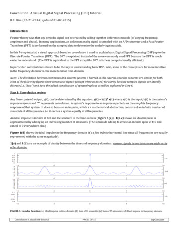
Signal processingSignals may have to be transformed in order to amplify or filter out embedded information methods to measure, characterise, model and simulate transmission channels mathematical tools that split common channels and transformations into easily manipulated building blocksdetect patternsprepare the signal to survive a transmission channelprevent interference with other signals sharing a mediumundo distortions contributed by a transmission channelcompensate for sensor deficienciesfind information encoded in a different domainTo do so, we also need3Analog electronicsPassive networks (resistors, capacitors,inductances, crystals, SAW filters),non-linear elements (diodes, . . . ),(roughly) linear operational amplifiersRUinLCUoutAdvantages: analog signal-processing circuitsrequire little or no power analog circuits cause little additional interferenceUinUinUout passive networks are highly linearover a very large dynamic rangeand large bandwidthsUout0 1/ LCω ( 2πf)Uin Uout1 RLtZt Uout dτ CdUoutdt4
Digital signal processingAnalog/digital and digital/analog converter, CPU, DSP, ASIC, FPGA.Advantages: noise is easy to control after initial quantizationhighly linear (within limited dynamic range)complex algorithms fit into a single chipflexibility, parameters can easily be varied in softwaredigital processing is insensitive to component tolerances, aging,environmental conditions, electromagnetic interferenceBut: discrete-time processing artifacts (aliasing)can require significantly more power (battery, cooling)digital clock and switching cause interference5Typical DSP applications communication systems consumer electronicsmodulation/demodulation, channelequalization, echo cancellationperceptual coding of audio and videoon DVDs, speech synthesis, speechrecognition music medical diagnostics synthetic instruments, audio effects,noise reductionmagnetic-resonance and ultrasonicimaging, computer tomography,ECG, EEG, MEG, AED, audiologygeophysicsseismology, oil exploration astronomy experimental physics aviation security engineeringVLBI, speckle interferometrysensor-data evaluationradar, radio navigationsteganography, digital watermarking,biometric identification, surveillancesystems, signals intelligence, electronic warfarecontrol systems, feature extractionfor pattern recognition6
SyllabusSignals and systems. Discrete sequences and systems, their types and properties. Linear time-invariant systems, convolution. Harmonic phasors are the eigenfunctions of linear time-invariant systems. Review of complex arithmetic. Someexamples from electronics, optics and acoustics.MATLAB. Use of MATLAB on PWF machines to perform numerical experimentsand visualise the results in homework exercises.Fourier transform. Harmonic phasors as orthogonal base functions. Forms of theFourier transform, convolution theorem, Dirac’s delta function, impulse combs inthe time and frequency domain.Discrete sequences and spectra. Periodic sampling of continuous signals, periodic signals, aliasing, sampling and reconstruction of low-pass and band-passsignals, spectral inversion.Discrete Fourier transform. Continuous versus discrete Fourier transform, symmetry, linearity, review of the FFT, real-valued FFT.Spectral estimation. Leakage and scalloping phenomena, windowing, zero padding.7Finite and infinite impulse-response filters. Properties of filters, implementation forms, window-based FIR design, use of frequency-inversion to obtain highpass filters, use of modulation to obtain band-pass filters, FFT-based convolution,polynomial representation, z-transform, zeros and poles, use of analog IIR designtechniques (Butterworth, Chebyshev I/II, elliptic filters).Random sequences and noise. Random variables, stationary processes, autocorrelation, crosscorrelation, deterministic crosscorrelation sequences, filtered randomsequences, white noise, exponential averaging.Correlation coding. Random vectors, dependence versus correlation, covariance,decorrelation, matrix diagonalisation, eigen decomposition, Karhunen-Loève transform, principal/independent component analysis. Relation to orthogonal transformcoding using fixed basis vectors, such as DCT.Lossy versus lossless compression. What information is discarded by humansenses and can be eliminated by encoders? Perceptual scales, masking, spatialresolution, colour coordinates, some demonstration experiments.Quantization, image and audio coding standards. A/µ-law coding, delta coding, JPEG photographic still-image compression, motion compensation, MPEGvideo encoding, MPEG audio encoding.Note: The last three lectures on audio-visual coding were previously part of the course “Information Theory and Coding”. A brief introduction to MATLAB was given in “Unix Tools”.8
ObjectivesBy the end of the course, you should be able to apply basic properties of time-invariant linear systems explain the above in time and frequency domain representations provide a good overview of the principles and characteristics of several widely-used compression techniques and standards for audiovisual signalsunderstand sampling, aliasing, convolution, filtering, the pitfalls ofspectral estimationuse filter-design softwarevisualise and discuss digital filters in the z-domainuse the FFT for convolution, deconvolution, filteringimplement, apply and evaluate simple DSP applications in MATLABapply transforms that reduce correlation between several signal sourcesunderstand and explain limits in human perception that are exploited by lossy compression techniques9Textbooks R.G. Lyons: Understanding digital signal processing. PrenticeHall, 2004. ( 45) A.V. Oppenheim, R.W. Schafer: Discrete-time signal processing. 2nd ed., Prentice-Hall, 1999. ( 47) J. Stein: Digital signal processing – a computer science perspective. Wiley, 2000. ( 74) S.W. Smith: Digital signal processing – a practical guide forengineers and scientists. Newness, 2003. ( 40) K. Steiglitz: A digital signal processing primer – with applications to digital audio and computer music. Addison-Wesley,1996. ( 40) Sanjit K. Mitra: Digital signal processing – a computer-basedapproach. McGraw-Hill, 2002. ( 38)10
Sequences and systemsA discrete sequence {xn } n is a sequence of numbers. . . , x 2 , x 1 , x0 , x1 , x2 , . . .where xn denotes the n-th number in the sequence (n Z). A discretesequence maps integer numbers onto real (or complex) numbers.We normally abbreviate {xn } n to {xn }, or to {xn }n if the running index is not obvious.The notation is not well standardized. Some authors write x[n] instead of xn , others x(n).Where a discrete sequence {xn } samples a continuous function x(t) asxn x(ts · n) x(n/fs ),we call ts the sampling period and fs 1/ts the sampling frequency.A discrete system T receives as input a sequence {xn } and transformsit into an output sequence {yn } T {xn }:. . . , x2 , x1 , x0 , x 1 , . . .discretesystem T. . . , y2 , y1 , y0 , y 1 , . . .11Properties of sequencesA sequence {xn } isabsolutely summable square summable Xn Xn xn xn 2 periodic k 0 : n Z : xn xn kA square-summable sequence is also called an energy signal, and Xn xn 2is its energy. This terminology reflects that if U is a voltageR supplied to a loadresistor R, then P U I U 2 /R is the power consumed, and P (t) dt the energy.So even where we drop physical units (e.g., volts) for simplicity in calculations, itis still customary to refer to the squared values of a sequence as power and to itssum or integral over time as energy.12
A non-square-summable sequence is a power signal if its average powerkX1 xn 2limk 1 2kn kexists.Special sequencesUnit-step sequence:un 0, n 01, n 0Impulse sequence: 1, n 00, n 6 0 un un 1δn 13Types of discrete systemsA causal system cannot look into the future:yn f (xn , xn 1 , xn 2 , . . .)A memory-less system depends only on the current input value:yn f (xn )A delay system shifts a sequence in time:yn xn dT is a time-invariant system if for any d{yn } T {xn } {yn d } T {xn d }.T is a linear system if for any pair of sequences {xn } and {x′n }T {a · xn b · x′n } a · T {xn } b · T {x′n }.14
Examples:The accumulator systemyn nXxkk is a causal, linear, time-invariant system with memory, as are the backward difference systemyn xn xn 1 ,the M-point moving average systemM 11 Xxn M 1 · · · xn 1 xnyn xn k M k 0Mand the exponential averaging systemyn α · xn (1 α) · yn 1 α Xk 0(1 α)k · xn k .15Examples for time-invariant non-linear memory-less systems:yn x2n ,yn log2 xn ,yn max{min{⌊256xn ⌋, 255}, 0}Examples for linear but not time-invariant systems: xn , n 0 xn · unyn 0, n 0yn x⌊n/4⌋yn xn · ℜ(eωjn )Examples for linear time-invariant non-causal systems:1(xn 1 xn 1 )29Xsin(πkω)· [0.5 0.5 · cos(πk/10)] xn k ·πkωk 9yn yn16
Constant-coefficient difference equationsOf particular practical interest are causal linear time-invariant systemsof the formxnyn b0 · xn NXk 1b0ynak · yn k a1x′nAddition:Multiplicationby constant:Delay:xnxnaxnyn 2z 1yn 3The ak and bm areconstant coefficients.xn 1z 1z 1 a3xn x′nayn 1 a2Block diagram representationof sequence operations:xnz 117orxnyn MXm 0bm · xn mz 1xn 1b0b1xnz 1k 0ak · yn k xn 2z 1xn 3b2b3ynor the combination of both:NXz 1MXm 0bm · xn mb0a 10b1 a1xn 1z 1b2xn 2z 1xn 3b3 a2 a3ynz 1yn 1z 1yn 2z 1yn 3The MATLAB function filter is an efficient implementation of the last variant.18
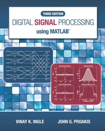
ConvolutionAll linear time-invariant (LTI) systems can be represented in the formyn Xk ak · xn kwhere {ak } is a suitably chosen sequence of coefficients.This operation over sequences is called convolution and defined as{pn } {qn } {rn } n Z : rn Xk pk · qn k .If {yn } {an } {xn } is a representation of an LTI system T , with{yn } T {xn }, then we call the sequence {an } the impulse responseof T , because {an } T {δn }.19Convolution examplesABCDEFA BA CC AA ED EA F20
Properties of convolutionFor arbitrary sequences {pn }, {qn }, {rn } and scalars a, b: Convolution is associative Convolution is commutative Convolution is linear The impulse sequence (slide 13) is neutral under convolution Sequence shifting is equivalent to convolving with a shiftedimpulse{pn d } {pn } {δn d }({pn } {qn }) {rn } {pn } ({qn } {rn }){pn } {qn } {qn } {pn }{pn } {a · qn b · rn } a · ({pn } {qn }) b · ({pn } {rn }){pn } {δn } {δn } {pn } {pn }21Can all LTI systems be represented by convolution?Any sequence {xn } can be decomposed into a weighted sum of shiftedimpulse sequences:{xn } Xk xk · {δn k }Let’s see what happens if we apply a linear( ) time-invariant( ) systemT to such a decomposed sequence:T {xn } T Xk ( ) Xk !xk · {δn k }( ) Xk xk · {δn k } T {δn } {xn } T {δn }q.e.d.xk · T {δn k } Xk !xk · {δn k } T {δn } The impulse response T {δn } fully characterizes an LTI system.22
Exercise 1 What type of discrete system (linear/non-linear, time-invariant/non-time-invariant, causal/non-causal, causal, memory-less, etc.) is:3xn 1 xn 2xn 3(a) yn xn (e) yn (b) yn xn 1 2xn xn 1(f) yn xn · en/14(c) yn 8Yxn ii 0(d) yn 21 (x2n x2n 1 )(g) yn xn · un(h) yn Xi xi · δi n 2Exercise 2Prove that convolution is (a) commutative and (b) associative.23Exercise 3 A finite-length sequence is non-zero only at a finite number ofpositions. If m and n are the first and last non-zero positions, respectively,then we call n m 1 the length of that sequence. What maximum lengthcan the result of convolving two sequences of length k and l have?Exercise 4 The length-3 sequence a0 3, a1 2, a2 1 is convolvedwith a second sequence {bn } of length 5.(a) Write down this linear operation as a matrix multiplication involving amatrix A, a vector b R5 , and a result vector c.(b) Use MATLAB to multiply your matrix by the vector b (1, 0, 0, 2, 2)and compare the result with that of using the conv function.(c) Use the MATLAB facilities for solving systems of linear equations toundo the above convolution step.Exercise 5 (a) Find a pair of sequences {an } and {bn }, where each onecontains at least three different values and where the convolution {an } {bn }results in an all-zero sequence.(b) Does every LTI system T have an inverse LTI system T 1 such that{xn } T 1 T {xn } for all sequences {xn }? Why?24
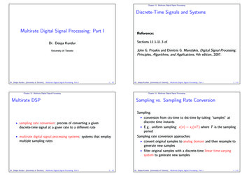
Direct form I and II implementationsxnz 1b0a 10b1 a1xn 1z 1b2 a2xn 2z 1b3 a3xn 3ynxnz 1a 10 a1yn 1 z 1yn 2z 1yn 3 a2 a3b0z 1z 1z 1ynb1b2b3The block diagram representation of the constant-coefficient differenceequation on slide 18 is called the direct form I implementation.The number of delay elements can be halved by using the commutativity of convolution to swap the two feedback loops, leading to thedirect form II implementation of the same LTI system.These two forms are only equivalent with ideal arithmetic (no rounding errors and range limits).25Convolution: optics exampleIf a projective lens is out of focus, the blurred image is equal to theoriginal image convolved with the aperture shape (e.g., a filled circle): Point-spread function h (disk, r h(x, y) 1,r2 π0, as)
Digital Signal Processing Markus Kuhn Computer Laboratory http://www.cl.cam.ac.uk/teaching/0809/DSP/ Lent 2009 – Part II Signals flow of information measured quantity that varies with time (or position) electrical signal received from a transducer (microphone, thermometer, accelerometer, antenna, etc.) electrical signal that controls a process