Transcription
.Math 623 - Computational FinanceBarrier option pricing using Finite Difference Methods (FDM)Pratik Mehtapbmehta@eden.rutgers.eduMasters of Science in Mathematical FinanceDepartment of Mathematics, Rutgers UniversityThis paper describes the implementation of a C program to calculate the value of a europeanstyle call option and a discretely sampled up-and-out barrier option on an underlying asset, giveninput parameters for stock price (s 100), strike price (k 110),volatility (v 30%), interestrate (r 5%), maturity (T 1 year), U 120 knock out usingclosed form solution, andFinite difference method. We compare the results of all these methods. The underlying stockprice is assumed to follow geometric brownian motion. [2].I.Here, N is the Normal Cumulative Distribution densityand the parameters, d and d are given byINTRODUCTIONIn this assignment we are pricing a European stylevanilla call option and discretely monitored barrier option (t 252) using closed form solution, and Finitedifference method.dS(t) (rS(t)dt σS(t)dW (t)(1)the solution to the above Stochastic Differential Equationis,1S(T ) S(0)e(r 2 σ2)T σW (T ) d d σ T 1xlog r σ 2 T (. 8)K2σ T1 The closed form solution to the option is implementedin the file BlackScholesFormulas.cpp and the formula isgiven below The output is as follows,Closed f orm option price 9.057(9)(2)III.BARRIER OPTIONSthe payoff for the call option is,(S(T ) k) (3)We also price an up-and-out barrier option. This can berepresented by,(S(T ) k) 1maxS(t) UII.(4)VANILLA CALL : CLOSED FORMBLACK-SCHOLES-MERTON(S(T ) k) 1max(S(t)) UHere, K is the strike price and S(T ) is the terminalstock price at the payoff date. The price of the underlyingat terminal time,T , is given by [3]1S(T ) S(0)e(r a 2 σ2)T σW (T )Barrier options are path-dependent options, with payoffs that depend on the price of the underlying asset atexpiration and whether or not the asset price crossesa barrier during the life of the option. There are twocategories or types of Barrier options: ”knock-in” and”knock-out”. ”Knock-in” or ”in” options are paid for upfront, but you do not receive the option until the assetprice crosses the barrier. This Knock-in can be represented by,(5)A closed form solution for the price of a European Calland Put is given by [3]c(t, x) xe aT N (d (T, x)) e rT KN (d (τ, x)) (6)andp(t, x) e rT KN ( d (T, x)) xe aT N ( d (τ, x)).(7)(10)”Knock-out” or ”out” options come into existenceon the issue date but becomes worthless if the assetprice hits the barrier before the expiration date. If theoption is a knock-in (knock-out), a predetermined cashrebate may be paid at expiration if the option has notbeen knocked in (knocked-out) during its lifetime. Thebarrier monitoring frequency specifies how often theprice is checked for a breach of the barrier. All of theanalytical models have a flag to change the monitoringfrequency where the default frequency is continuous.Up-and-out options are represented as(S(T ) k) 1S(t) U(11)
2The closed form solution to the up and out barrier optionis implemented in the file ClosedFormUpOutCall.cpp andthe formula is given belowCup C(t, S(t)) S(t)e d(T t) N (x1 ) ke r(T t) N (x1 σ T t) H 2λS(t)e d(T t) N (x1 )() (N (y) N ( y))S(t) H 2λ 2ke r(T t) N (x1 ()(N ( y) σ T t)S(t) N ( y1 σ T t)The algorithm to compute the finite difference solutionis given below[6](12)(13)(14)(15)(16)The output is as follows,Closed f orm option price 0.0524IV.(17)Divide the solution space into 2D meshF or i 0 to asstetstepsS(i) i assetstepsV (i, 0) CallP ayof f (S(i))Def ine A B and Cnext iF or k 0 to timestepsF or i 0 to asstetsteps(25)(26)(27)(28)(29)(30)(31)(32)kkVik 1 Aki Vi 1 (1 Bik )Vik Cik Vi 1next iV (0, k 1) 0(33)(34)(35)VIk IδS Strike e( rkδt)next k(36)(37)NUMERICAL SOLUTION TO PDE USINGFINITE DIFFERENCE METHODThere are many cases where the PDE cannot be analytically solved or the solution is very tedious. In thesecases we can easily approximate the solution using numerical methods like Finite difference. Finite DifferenceMethod generally seeks to approximate the solution tosome PDE. Generally, the statement of a problem hastwo parts.Conditions: a Partial Differential Equation (PDE),boundary conditions, constraints, and so on.Data: initial values, final values (e.g. a payout function), boundary values, and so on.We use the above algorithm to price a call option,F inite Dif f erence call option price 9.077To price the up-and-out barrier option, we have to doa couple of changes, The first change is that we haveto reduce the number of asset steps so that the valuebecomes 0 for any price above U. And the second is theboundary condition, the upper boundary at S 120, thevalue of the option is forced to be 0.F inite Dif f erence barrier option price 0.056 (39)The Black and Scholes formula to calculate the value ofan option is derived by solving the Black-Scholes partialdifferential equation: f1 2f f rS σ 2 S 2 2 rf ,(18) t S2 SWe can approximate the above PDE using Forward/Backward/Central difference. uu(x, t t) u(x, t) , t t(19)and 2uu(x x, t) 2u(x, t) u(x x, t) ,2 x x2(20)We can write the Black Scholes PDE using Finite difference askkVik 1 Aki Vi 1 (1 Bik )Vik Cik Vi 11A (σ 2 i2 (r d)i)δt2B (σ 2 i2 r)δt1C (σ 2 i2 (r d)i)δt2(38)V.ANSWER TO THE QUESTIONSQ1We have used explicit finite difference and we found thatwhen the time steps T 252 and Space intervals N 50,the value of the vanilla and barrier options are in agreement to the closed form solutions. But explicit FDmethod has some disadvantages. First of all, the methoddoes not converge and is stable all the time. The convergence and stability depends on the value of T (Timeintervals) and N (Space intervals). Also there is a dependence of δt and δs on each other. They cannot beindependently varied .Paul WIlmott shows that for convergence and stablity the following conditions should memet,(21)δs 2a b (40)(22)(23)(24)andδt 1σ2 I 2(41)
3Using the above conditions we find that,δt 230(42)We have tried a combination of step sizes to test robustness of the stability and convergence criteria. We calculated the option prices for various δt and δs. We variedδt from 100 to 500 and δs from 2 to 30. We find thatthe results blow up when δt is less than 200 (approx)and when δs is greater than 50 . We have tabulatedthe results (below).Q2If we vary Smax , we also inadvertently change δs, if weincrease Smax without adjusting δs, we get inaccurateanswers. Both of them will have to vary accordingly. Inout C code, we varied Smax and kept δs constant. Wefind that for δs 4, Smax 240 blows the answer. Wehave tabulated the results.VI.BENCHMARKINGWe have used many spreadsheet based models tobenchmark our results. The summary go the benchmarking is given below and is also tabularised below. We haveused Excel spreadsheets by Haug and Black and Numerixto price. The benchmarked results are in agreement withthe results obtained from C . The results are,N umerix option price vanilla 9.08N umerix up in andout 0.05Haug vanilla call 9.05Haug up and out call 0.05(43)(44)(45)(46)
4TABLE I: Vanilla and Asian Call pricing using Methods for S(0) 100 and K 110OptionEuropean Vanilla CallBarrier (Up-and-out) CallClosed Form9.050.052Finite Difference9.070.056Haug9.0570.05TABLE II: Effect of varying δsStrata size4510203060Vanilla Call9.0779.0438.959.055.620.94Barrier call0.0560.0450.00740.0760.00790.002TABLE III: Effect of varying δtStrata size100200300400500Vanilla Call1.5e 0279.0789.0769.0759.074Barrier call0.0670.0580.0550.05380.0529TABLE IV: Effect of varying SmaxSmax140180200240300Vanilla Call9.059.109.0779.06-4.7e 059Barrier call0.050.0560.05640.0560.0564Numerix9.080.05
5
6FIG. 2: Barrier
7[1] re[2] M.S. Joshi, C design Patterns and Derivative Pricing,(Wiley 2008).[3] S.E. Shreve, Stochastic Calculus for Finance II ContinuousTime Models, (Springer, 2004).[4] Wikipedia page for low discrepancy sequence[5] I M Sobol, USSR comp. Math[6] Jonathan Goodman,Courant Institute of MathematicalScience, NYU[7] www.cecs.csulb.edu/ ebert/teaching/lectures/552/[8] rss.acs.unt.edu/Rdoc/library/fExoticOptions[9] BarrierOptions
fanw/download/lecture [2] M.S. Joshi, C design Patterns and Derivative Pricing, (Wiley 2008). [3] S.E. Shreve, Stochastic Calculus for Finance II Continuous Time Models, (Springer, 2004). [4] Wikipedia page for low discrepancy sequence [5] I M Sobol, USSR comp. Math [6] Jonathan Goodman,Courant Institute of Mathematical Science, NYU