Transcription
Pattern Recognition Letters 31 (2010) 1489–1497Contents lists available at ScienceDirectPattern Recognition Lettersjournal homepage: www.elsevier.com/locate/patrecIncorporating scale information with cepstral features: Experimentson musical instrument recognitionMarcela Morvidone a,b, Bob L. Sturm b, Laurent Daudet c,*aLaboratoire de Physique Théorique et Modélisation, Université de Cergy-Pontoise, Site de Saint-Martin, Pontoise, 2 Av. Adolphe Chauvin, 95302 Cergy-Pontoise, FranceInstitut Jean Le Rond d’Alembert (IJLRA), Équipe Lutheries, Acoustique, Musique (LAM), Université Pierre et Marie Curie (UPMC) – Paris 6, UMR 7910, 11,rue de Lourmel, 75015 Paris, FrancecInstitut Langevin (LOA), Université Paris Diderot – Paris 7, UMR 7587, 10, rue Vauquelin, 75231 Paris, Franceba r t i c l ei n f oArticle history:Available online 4 January 2010Keywords:Audio signal classificationSparse decompositionsTime–frequency/time-scale featuresMusical instrument recognitiona b s t r a c tWe present two sets of novel features that combine multiscale representations of signals with the compact timbral description of Mel-frequency cepstral coefficients (MFCCs). We define one set of features,OverCs, from overcomplete transforms at multiple scales. We define the second set of features, SparCs,from a signal model found by sparse approximation. We compare the descriptiveness of our featuresagainst that of MFCCs by performing two simple tasks: pairwise musical instrument discrimination,and musical instrument classification. Our tests show that both OverCs and SparCs improve the characterization of the global timbre and local stationarity of an audio signal than do mean MFCCs with respectto these tasks.! 2010 Elsevier B.V. All rights reserved.1. IntroductionFor speech signal processing tasks, for instance, speaker verification (Bimbot et al., 2004; Ganchev et al., 2005), or speech recognition (Rabiner and Juang, 1993), the use of Mel-frequency cepstralcoefficient features (MFCCs) has proven extremely effective because they provide compact and perceptually meaningful descriptions of the distribution of formants. Though the source-filtermodel does not fit every manner of sound production, the use ofMFCCs has also benefited tasks involving discrimination betweentimbres in non-speech signals, such as musical instrument recognition (Essid et al., 2006; Joder et al., 2009), musical fingerprinting(Casey et al., 2008), and environmental sound classification (Cowling and Sitte, 2003; Couvreur and Laniray, 2004; Defréville et al.,2006). To improve performance in many of these tasks, MFCCsare often combined with other features, such as the set of timeand frequency-domain features specified in the MPEG-7 audiostandard (Manjunath et al., 2002).To describe a signal with time-varying statistics in terms ofMFCCs, one computes them in a time-localized fashion over shortwindows during which the signal is assumed to be stationary,e.g., typically 20–30 ms windows spaced every 10 ms for speechsignals. This duration is reasonably based for speech processingon the physics of speech production (Rabiner and Juang, 1993),* Corresponding author. Tel.: 33 (0) 1 40 79 46 92; fax: 33 (0) 1 40 79 44 68.E-mail address: laurent.daudet@espci.fr (L. Daudet).0167-8655/ - see front matter ! 2010 Elsevier B.V. All rights reserved.doi:10.1016/j.patrec.2009.12.035i.e., the human voice is limited in the number of timbres it can produce per unit time. However, the assumption of stationarity over asingle short-time duration for music signals is often unreasonableif we consider the phenomena that occur over a range of differenttime-scales, for instance, transients, vibrato, tremolo, sustainedharmonics, etc. Furthermore, many phenomena can occur simultaneously, which are inseparable in MFCCs by their non-linearity. Itdoes not make sense to think that the MFCCs of a portion of a music signal that contains a strong transient are meaningful otherthan to say the power spectral density is more wideband than inanother segment. In such a case, it would be more perceptually relevant to separate the description of the transient (Herrera-Boyeret al., 2003) from that of the rest of the local signal.For recognition tasks involving signals with phenomena occurring over multiple time-scales, such as musical signals (Cowlingand Sitte, 2003; Couvreur and Laniray, 2004; Defréville et al.,2006; Aucouturier et al., 2007; Casey et al., 2008; Joder et al.,2009), MFCCs generated using a single window size and uniformtranslations must be suboptimal with respect to their descriptiveness, than are features computed with considerations for the diversity of time-scales present. What is desired for such signals then isa set of features that have the compact descriptiveness of MFCCswhile taking into account the local statistics of the signal so thatone may better distinguish its contents. In other words, for signalcontent having slowly varying statistics it is unnecessary to compute MFCCs every 10 ms using a 30 ms window; and for signal content occurring over short time-scales we should avoid ‘‘smearing”its influence over a large window. We want to separate the
1490M. Morvidone et al. / Pattern Recognition Letters 31 (2010) 1489–1497influence of these contents so that the signal features are more local and specific, and can better characterize a signal.In this paper we address these issues by defining and testingtwo sets of novel features that provide information about the spectral shape of a signal, as well as the time-scales involved. One set offeatures, OverCs (pronounced ‘‘over seas”), basically aggregates theMFCCs computed from redundant transforms performed at multiple scales. The other set of features, SparCs (pronounced ‘‘sparseas”), looks at the distribution of energy among frequency andscale of a sparse model of a signal found using sparse approximation and a multiscale time–frequency dictionary. Sparse approximation methods have been shown to provide efficient andmeaningful parametric representations adapted to audio data(Mallat and Zhang, 1993; Gribonval and Bacry, 2003; Daudet,2006; Leveau et al., 2008), where small-scale atoms are used tomodel transients, and large-scale atoms are used for tonals. Thisprovides a level of source separation that can remove the influenceof short-scale phenomena on the spectral description of large-scalephenomena. Though sparse approximation has a large computational complexity, we consider the case where a database of audiosignals has already been decomposed, for instance, in its compression (Ravelli et al., 2008). We expect that both of these features willbe more discriminative than mean MFCCs for content recognitiontasks because they consider multiple scales. We test this by comparing the discriminative ability of these features with those ofmean MFCCs in two simple tasks: pairwise musical instrument discrimination, and musical instrument classification. For each ofthese features, we select a small number of coefficients to comparewith the mean MFCCs at a fixed dimensionality. The signals we useare excerpted from real musical recordings, and have been used inother automatic classification works (Essid, 2005). We find that forboth tasks our proposed features perform better than the meanMFCCs.The rest of this paper is organized as follows. In Section 2 we review MFCCs, and then sparse approximation with time–frequencydictionaries. We define our new features in Section 3, and providesome examples. In Section 4 we detail our experiments and discussthe results and their significance. Finally, we conclude with adescription of ongoing work in several directions.2. BackgroundIn this section, we review MFCCs, as well as sparse approximation using greedy iterative methods with a time–frequencydictionary.2.1. Review of Mel-frequency Cepstral Coefficients (MFCCs)The cepstrum models the distribution of spectral energy in atime-domain signal. Given a real length-N discrete signal, x, defined over 0 6 n N, and its discrete Fourier transform (DFT),X ¼ DFTfxg, its real cepstrum is defined (Rabiner and Juang,1993)N 11 Xc½l# , DFT 1 flog jXjg ¼ pffiffiffilog jX½k#jej2pkl N ;N k¼0l ¼ 0; 1; . . . ; N 1ð1Þwhere the logarithm is used to separate the filtering from the excitation signal. The magnitudes of the cepstrum provide a descriptionof the spectral shape of x independent of a wideband excitation signal. Because this fits the manner of speech production, the cepstrum has been very successful for tasks of speaker and speechrecognition (Rabiner and Juang, 1993).To create a less redundant and perceptually-relevant representation of the spectral shape of x, one finds the energies in frequencybands according to perceived pitch by the Mel-frequency scaling,which maps a frequency f (Hz) to Mels by /ðf Þ ¼ 1127lnð1 þ f 700Þ. The filterbank we use has L ¼ 40 overlapping bandswith triangular magnitude responses, weighted such that each hasequal area, beginning at a low frequency of 133.33 Hz, and endingat the high frequency of 6853.84 Hz (Ganchev et al., 2005). The first13 filters are linearly spaced every 66.67 Hz with a bandwidth of133.33 Hz, and weighting 0.015. The last 27 filters have center frequencies that are logarithmically spaced from 1073.4 Hz to6413.59 Hz. The center frequencies of the filters are given byfc ðlÞ ¼"133:33 þ 66:66l;l ¼ 1; 2; . . . ; 131073:4ð1:0711703Þðl 14Þ ; l ¼ 14; 15; . . . ; 40:ð2ÞEach filter ðl ¼ 1; 2; . . . ; 40Þ is given byHl ½k# ,80;0 6 kF s N fc ðl 1Þ kF s N fc ðl 1Þ ; f ðl 1Þ 6 kF N f ðlÞ cscfc ðlÞ fc ðl 1ÞkF s N fc ðlþ1Þ ; fc ðlÞ 6 kF s N fc ðl þ 1Þ f ðlÞ f ðlþ1Þ : c c0;fc ðl þ 1Þ 6 kF s NF sð3Þ;where F s is the Nyquist sampling rate (Hz), fc ð0Þ ,133:33; fc ð41Þ , 6853:84, and the band-dependent magnitudefactors fal g are given byal ,(0:015;1 6 l 6 132;fc ðlþ1Þ fc ðl 1Þ14 6 l 6 40:ð4ÞWith this filter bank, we compute the Mel-frequency cepstralcoefficients (MFCCs) by a discrete cosine transform (DCT)ccM ½m# , bL ðmÞLP 1XXl¼1k¼0!log jX½k#al Hl ½k#j cos%# &mp1;l 2Lð5Þdefined for 0 6 m L, and where the normalization factor is definedbR ðyÞ ,(pffiffiffi1 R;y¼0pffiffiffiffiffiffiffiffi2 R; 1 6 y 6 R:ð6ÞFor speech and audio data, the DCT provides a satisfactory decoupling of the components of their log magnitude spectra (Logan,2000). Since speech and audio signals are non-stationary, MFCCsare calculated in practice using overlapping sliding windows. Wedefine the short-time MFCCsccM ½m; p# , bL ðmÞLN 1XXl¼1k¼0!log jX½k; p#al Hl ½k#j cos%# &mp1;l 2Lð7Þfor 0 6 m L, and where the DFT of x localized at time p is definedP 11 XX½k; p# , pffiffiffix½n þ p#w½n#e j2pkn P ;P n¼00 6 k 6 P 1;ð8Þfor time shifts 0 6 p N P, and a real window w that is non-zerofor 0 6 n P, and that satisfiesP 11 Xpffiffiffijw½n#j2 ¼ 1:P n¼0ð9ÞIn speech recognition and music processing it is typical to use windows of length 20 – 30 ms, over which durations the signal can besaid to be approximately stationary. These windows are usuallyplaced at translations of half their duration. For speech signals, onlythe first M ¼ 13 coefficients are typically kept (Rabiner and Juang,1993), excepting the term at m ¼ 0 since it reflects only the shortterm energy of the signal.
1491M. Morvidone et al. / Pattern Recognition Letters 31 (2010) 1489–14972.2. Sparse Approximation with Time–Frequency DictionariesSparse approximation attempts to find a small subset of Matoms in a dictionary D ¼ fg c gc2C to approximate the length-Nfunction x to some specified maximum error ! P 0, e.g.,'2'''MX'min M subject to 'x acm g cm '' 6 !;''m¼12ð10ÞMwhere fcm gMm¼1 ( C, and facm gm¼1 is the set of weights associatedwith the M atoms selected in D. The term sparse refers to the desirable property by which the number of atoms selected M ) N, thedimension of the signal. Usually, jCj * N such that many possiblesolutions exist.Various methods have been proposed to solve (10), e.g., a greedy iterative strategy (Mallat and Zhang, 1993), or convex optimization with a relaxed sparsity constraint (Chen et al., 1998). Themethod we use in this paper is Matching Pursuit (MP) (Mallatand Zhang, 1993). MP selects the ðM þ 1Þth atom from D by thecriterioncMþ1'2''hRM x; g c ig c 'jhRM x; g c ij'' M¼ arg min 'R x ¼argmax;'c2C 'c2Ckg c k2kg c k22 '2ð11Þwhere the inner product between two real length-N functions x andy is definedhx; yi ,N 1Xð12Þand the Mth-order residual signal is definedMXm¼1acm g cm :ð13ÞMP defines the ðM þ 1Þth weight byacMþ1 ,hRM x; g cMþ1 ikg cMþ1 k22ð14Þ:In this way, MP iteratively selects the atom that maximally reducesthe ‘2 -norm of an intermediate residual, beginning with R0 x ¼ x.Various dictionaries have been used in the sparse approximation of speech and audio signals, such as Gabor time–frequencyatoms (Mallat and Zhang, 1993), harmonic atoms (Gribonval andBacry, 2003; Leveau et al., 2008), or unions of bases, such as cosineand wavelet bases (Daudet, 2006), and multiscale cosine bases(Ravelli et al., 2008). In this work, we use time–frequency atomsthat have a single modulation frequency x and phase /, time scales, and time shift u. Considering that an element c 2 C is the quadruple cm ¼ ðsm ; um ; xm ; /m Þ, a real length-N time–frequencyatom is definedg cm ½n# , gs (samples/ms)Du (samples/ms)Df 121.510.85.42.73. Incorporating Scale Information with Cepstral FeaturesWe now define two sets of novel features, OverCs and SparCs,that combine a time-domain scale characterization of a signal witha frequency-domain spectral characterization. For OverCs, we useovercomplete transforms performed at multiple scales. For SparCs,we use a signal model found by sparse approximation and a multiscale time–frequency dictionary. Sparse approximation allows aminimum amount of source separation between phenomena thatoccur over different time scales. Though OverCs are less computationally intensive than SparCs, it does not allow for any sourceseparation.3.1. OverCs: MFCC-like Features from Overcomplete Transformsx½n#y½n#;n¼0RM x , x Table 1Dictionary parameters of a scaled, shifted, and modulated Gaussian lowpass function:scale s, time resolution Du , and frequency resolution Df . Durations are specific to asampling rate F s ¼ 44100 Hz.# n umcosðxm n þ /m Þ;sm0 6 n N;ð15Þwhere gðtÞ is a continuous prototype lowpass function, for instancea Gaussian window. The dictionary specified by Table 1 containsatoms of scale 128 samples located at translations that are integermultiples of 32 samples i.e., um ¼ 32l; l 2 Z, and with modulationfrequencies that are positive integer multiples of 43.1 Hz, i.e.,xm ¼ 2pl43:1 F s ; l 2 Zþ (up to the Nyquist frequency pF s ). Whenthe dictionary D is complete, then limM!1 kRM xk22 ¼ 0, i.e., the representation converges such that the error becomes zero (Mallatand Zhang, 1993). In this article, we use MP Toolkit (Krstulovicand Gribonval, 2006) and Gaussian lowpass functions.We generate OverCs by first computing short-time MFCCs (7)using windows of multiple scales. The parameters of the windowswe use are the same as for the overcomplete dictionary detailed inTable 1. This means that we essentially project x onto all atoms ofthis dictionary, and then use these values to compute mean MFCCsfor each scale. Let us define ccM ½m; p; s# to be (7) computed using awindow scale 128 2ðs 1Þ , which are the L MFCCs of x over the timeregion ½p; p þ 128 2ðs 1Þ Þ. Now we define the set of short-timeMFCCsCs;! , fccM ½m; p; s# : ccM ½0; p; s# !;1 6 m 40g;ð16Þfrom time regions of scale index s in x with energy greater than! P 0 (to avoid signal frames near to silence), and where we haveexcluded all m ¼ 0 cepstral coefficients since they only contain energy information. We then form averages of this setccM ½m; s# ,1 XccM ½m; p; s#;jCs;! j p2Cs;!ð17Þwhere p 2 Cs;! means those p that exist in Cs;! . In other words, weaverage all contributions in cepstral index m and scale index s overthe short-time frames of size s. Finally, since there will be redundancy across scales in each cepstral index, we perform a DCT inthe scale direction to generate the OverCs:f½m; z# , b8 ðzÞ8Xs¼1ccM ½m; s# cos%# &ðz 1Þp1;s 28ð18Þfor 1 6 z 6 8, and using the normalization factor (6).3.2. SparCs: MFCC-like Features from Sparse ModelsConsider that we have approximated x by M atoms selectedfrom D by MP, thus producing an M-order model (10). We first separate the M atoms in the sparse model based on their modulationfrequency and scale parameters. Let us associate each atom withan integer and define this index set M , f1; 2; . . . ; Mg. Thus, atomm 2 M has parameters ðsm ; um ; xm ; /m Þ. We define the following
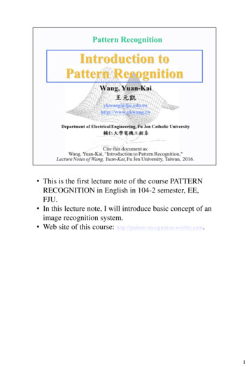
1492M. Morvidone et al. / Pattern Recognition Letters 31 (2010) 1489–1497mappings from the scale-frequency space of the model. For the dictionary specified in Table 1, we map each atom scale to an integerbySðsÞ , 1 þ log2 ðs 128Þ; s 2 f128;256;512; 1024; 2048; 4096; 8192;16384g:ð19ÞBased on the 40-band filterbank described in Section 2.1, we definethe modulation frequency mappingWðxÞ ,"l;40;fc ðl 1Þ 6 Xx fc ðl þ 1Þ;1 6 l 6 39fc ð40Þ 6 Xx fc ð41Þ;ð20Þwhere X , F s 2p, and the center frequencies are given by (2). Now,we define the index set of atoms in the sparse model that have somescale index r and modulation frequency index l asMlr , fm 2 M : Wðxm Þ ¼ l;Sðsm Þ ¼ rg:ð21ÞNote that there is no longer any notion of where in time a givenatom exists.From the set fMlr : 1 6 l 6 40; 1 6 r 6 8g, we accumulate themagnitude weights as a function of modulation frequency andscale:X½l; r# ,Xm2Mlr( (al Hl ðxm Þ(acm (;ð22Þwhere the filter weights fal g are given by (4), and we define, similarto (3),Fig. 1. ccM ½m; s# (17) and j log Xðr; lÞj (22) for two musical instruments playing a chromatic scale from C5 to B5.
1493M. Morvidone et al. / Pattern Recognition Letters 31 (2010) 1489–14978 Xx f ðl 1Þc ; fc ðl 1Þ 6 Xx fc ðlÞ fc ðlÞ fc ðl 1ÞXx fðlþ1ÞcHl ðxÞ ,; fc ðlÞ 6 Xx fc ðl þ 1Þ ;fc ðlÞ fc ðlþ1Þ :0;elseð23Þto weight the contribution of the atom to the lth frequency bin ofthe relevant scale index. We take the two-dimensional DCT ofX½l; r#, which, for this dictionary of 8 scales and filterbank of 40bands, is definedn½m; z# ,40 X8Xl¼1r¼1zz# &%# &ðm 1Þp1ðz 1Þp1b8 ðzÞ cos;cosr l 22408zz# n½m; z# , fiffiffiffiffiffiffiffiffi :P40 ffiP82m¼1z¼1 jn½m; z#jð25ÞSparCs are very fast to compute if a sparse decomposition is alreadyavailable.3.3. Examples of SparCs and OverCsX½l; r# , b40 ðmÞ,z%for 1 6 m 6 40 and 1 6 z 6 8, with the normalization factors defined by (6). Finally, we create the SparCs by setting n½1; 1# ¼ 0,and normalizing the rest:ð24ÞFig. 1(a) and (c) show the magnitude mean short-time MFCCs(17) for two different musical audio signals recorded from aclarinet and trumpet (IOWA, 2009). Each instrument plays 40Fig. 2. OverCs jf½m; z#j (18) and SparCs j n½m; z#j (25) from data in Fig. 1. Mean MFCCs of these two signals are shown in Fig. 3.
1494M. Morvidone et al. / Pattern Recognition Letters 31 (2010) 1489–1497recordings. For example, there exist double and triple stops inthe violin and cello examples, chords in the guitar and piano examples, pitch bends in the clarinet, as well as reverberation. We summarize our database in Table 2.We create the SparCs feature database using the dictionary defined in Table 1 with a Gaussian window, to the order M where thesignal-to-residual energy ratio reaches 20log10 ðkxk2 kRM xk2 Þ ¼ 30dB. We create the OverCs feature database with the same parameters as in Table 1. From these features, we select three differentsubsets of 13 ðm; zÞ features:ascending chromatic scale (C5 to B5), lasting 32 s (
We define the second set of features, SparCs, from a signal model found by sparse approximation. We compare the descriptiveness of our features against that of MFCCs by performing two simple tasks: pairwise musical instrument discrimination, and musical instrument classification. Our tests show that bo