Transcription
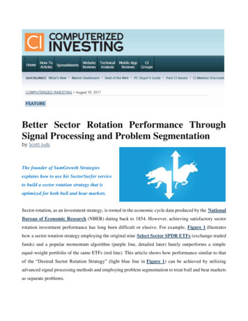
Better Sector Rotation Performance ThroughSignal Processing and Problem Segmentationby Scott JudsThe founder of SumGrowth Strategiesexplains how to use his SectorSurfer serviceto build a sector rotation strategy that isoptimized for both bull and bear markets.Sector rotation, as an investment strategy, is rooted in the economic cycle data produced by the NationalBureau of Economic Research (NBER) dating back to 1854. However, achieving satisfactory sectorrotation investment performance has long been difficult or elusive. For example, Figure 1 illustrateshow a sector rotation strategy employing the original nine Select Sector SPDR ETFs (exchange-tradedfunds) and a popular momentum algorithm (purple line, detailed later) barely outperforms a simpleequal-weight portfolio of the same ETFs (red line). This article shows how performance similar to thatof the “Desired Sector Rotation Strategy” (light blue line in Figure 1) can be achieved by utilizingadvanced signal processing methods and employing problem segmentation to treat bull and bear marketsas separate problems.
Figure 1. Comparison of Two Sector Rotation Strategies vs. an Equal-Weight PortfolioMarket CharacterThe conventional theory underlying sector rotation strategies is that markets predict the state of theeconomy typically three to six months in advance and that different sectors naturally perform betterduring particular portions of the economic cycle, as suggested by Figure 2. Although this model impliesthere’s an orderly sequence of market sectors and economic phases, sector performance has clearly beenstrongly affected by the introduction of new technologies that don’t wait their turn in the cycle to shine.Figure 2. Presumed Tie Between Market Cycle and Economic Cycle
It’s doubtful that Steve Jobs waited for this chart to tell him it was his turn before saying “And one morething—this is an iPhone.” Punctuated events such as elections, wars, political/monetary policy andnatural disasters don’t wait their turn either to change the direction or focus of the economy.Furthermore, the 2008–2009 financial crisis demonstrated that all sectors can suddenly becomecorrelated, simultaneously crashing and later rising together, as illustrated in Figure 3. Performing wellduring this period clearly requires something other than ordinary sector rotation.Figure 3. Correlated Market Sectors During the 2008–2009 Financial CrisisCompounding the problem further, bear market volatility is typically twice that of a bull market—a matter not addressed by ordinary momentum algorithms that often results in spurious trade alerts.Finally, even though it’s well understood that other asset classes perform better during a market crash,it is difficult to employ that knowledge well in a sector rotation strategy. In the process of addressingthese shortcomings of ordinary sector rotation here, we build on the principles presented in the January2017 CI article entitled “Using Asset Class Rotation to Reduce Risk and Increase Return.”
A Holistic SolutionWhen the first motorized carriage was designed, it was thought to be wonderful—at least until wedecided it also needed to run well in rain and snow, have tougher tires, air conditioning, locks and aradio. Attaching a simple engine to a frame with wagon wheels left much to be desired. Similarly, themost common and rudimentary of trend filters, the rectangular 12-month SMA (simple movingaverage), is far from optimum for determining which of a set of sector funds should be owned.Stepping back for a moment to review the nature of the problem as depicted by the sector trend chartof Figure 4, a few interesting things are observed:1. The S&P 500 (bold white line), is always flanked by sectors doing better or doing worse, asshould be expected because the S&P 500 is composed of all sectors.2. The waves generally have much in common—with the exception of bond and Treasury fundswhich typically have a mind of their own.3. There are funds on the left with high trends that a decade later have low trends, and viceversa, but there is no observable pattern of a grand, gradual rotation.Figure 4. Trends (Smoothed Monthly Return) for S&P 500, Sectors, Bonds & TreasuriesIt’s clear that to “win the game” of sector rotation, one must first and foremost do an excellent job ofowning the trend leader. However, because bear markets have quite a different character, attempting totreat bull and bear markets as one homogeneous problem results in disappointing performance, withperiods of underperformance that can easily last longer than one’s patience. A holistic sector rotationsolution requires solving three problems:1. optimizing bull market sector rotation,2. employing a market direction indicator to determine when it is a bull or bear market, and3. integrating a separate bear market strategy.
None of these are trivial when better performance is the objective. After examining these three topics,we employ them in a strategy using the original nine Select Sector SPDR ETFs.Improving Momentum IndicatorsSector rotation performance depends on extracting the momentum signal buried in noisy market data.In signal processing science, everything except for the desired signal is considered noise because insome form it degrades signal detection. For example, if the object is to find ETFs with momentum betterthan the S&P 500, then the process requires subtracting the S&P 500 daily returns from the ETF’s dailyreturns to remove the “common mode market noise,” and then subsequently apply a moving averagefilter to reduce remnant short-term noise. In this example, the S&P 500 itself is considered baselinemarket noise that must be removed. Although momentum in market data was formally found in1993 and confirmed in 2008, practitioners have long struggled to build satisfying momentum strategies.In this author’s opinion, satisfaction is proportional to the probability of making an outstandinginvestment decision.National Medal of Science recipient Claude Shannon’s 1948 theorem proved that the probability of asignal leading to a correct decision is directly proportional to its signal-to-noise ratio. An excellentanalogy is the probability of correctly hearing your honey-do list from a soft-spoken spouse in a noisycafé. Rewards are definitely better when you get it right. Figure 5 provides a visual illustration of high,medium and low signal-to-noise ratio (S/N). The size of the sine wave signal is constant in all three, butthe size of the noise changes. The signal and noise RMS values (root mean square—like standarddeviation) are used to calculate the ratio. It is common to state the ratio in decibels (dB), which is givenby:S/N(dB) 20 Log10(RMS(Signal)/RMS(Noise))When the signal and noise are the same sizes, the ratio is 1.00, which translates to 0.0dB. When thesignal is 3.16 times larger than the noise it is 10dB, and when 3.16 times smaller it is –10dB. It’s prettyeasy to see that the sine wave becomes reasonably discernable when the S/N 0dB or better and easilybecomes unrecognizable when buried in noise larger than itself.
Figure 5. Signal-to-Noise Ratio Visual ExampleThus, optimizing sector rotation performance requires pulling out all the stops to improve the signal-tonoise ratio of the momentum (trend) signal. When the signal and noise are similar in size, a 30%reduction in noise produces about a 30% improvement in the probability of buying the best fund —andthat is significant when your IRA is at stake! In the field of signal processing, the two most importantmeans of improving the signal-to-noise ratio are 1977 Nobel laureate J. H. Van Vleck’s matched filtertheory, and 1833 Royal Society fellow Samuel H. Christie’s differential signal processing method.Let’s examine each of these.Van Vleck’s matched filter theory can be used to optimize the momentum filter shape and duration toimprove the signal-to-noise ratio. The shape and duration of a filter determine what portions of the noisespectrum pass through the filter and what portions are blocked. It is referred to as a matched filterbecause in the frequency domain the optimum noise filter matches the signal’s frequency spectrum —the same principle used for tuning in a radio station. The frequency domain shape of the filter can betranslated to the time domain via the Laplace transform to instead show us the filter’s impulseresponse, which is what we are more accustomed to viewing when charting an SMA (simple movingaverage) or EMA (exponential moving average)filter.
Figure 6 illustrates a broad array of candidate momentum filters having different shapes and durations.The popular SMA-252 filter (green) averages 252 market days (one year) of equally weighted dailyreturn data over the period. The EMA-125 filter (top red) has an exponentially declining weight for datathe older it gets. Its 125-day time constant causes the weighting at day 125 (one-half year) to be 1/e 36.8% (where e is the base of the natural logarithm and has a value of 2.71828). A DEMA filter (blue,double exponential moving average) is sometimes referred to as a second-order EMA filter because thedata is doubly smoothed by passing it through the EMA filter twice.Figure 6. SMA, EMA and DEMA Filters With Multiple Shapes and DurationsRemarkably, the most common filter utilized in academic momentum research papers is the simplisticSMA-252 (although variations such as six months of duration, or skipping the most recent month areoccasionally employed). They have apparently never asked, “what are the chances that nature wouldhand us such a simple equally weighted (rectangular shape), exactly one-year duration filter as theoptimum solution?” I would suggest that the chances are about the same as the boxy Model-T Fordturning out to be the lowest wind resistance body design for efficient freeway driving. The SMA maybe an intellectually easy place to start, but matched filter theory shows us that the optimum filter shapeis neither the SMA, nor the EMA, but is actually more like the DEMA filter, as confirmed by strategydesign performance.Unfortunately, there is no single answer to the question of which DEMA filter duration is best. Whenconsidering the differences in character of diverse sets of asset classes (such as Treasuries, bonds,
utilities, REITs, commodities, sectors, regions and countries), it should not be surprising that theoptimum filter shape and duration depend not only on the asset class but also on the mix of asset classesthe strategy is tasked with considering. Although a broad range of filter shapes and durations is requiredfor broad functionality, the SMA shape is not among them. The reason the SMA turns out to be a poormomentum filter choice can be best understood by considering the basic idea behind matched filters.What it tells us is that on balance the SMA is including more noise than is necessary for the momentuminformation it is extracting from the data.Consider that the momentum signal is actually a predictor of near future performance (i.e., the expectedreturn next month). We want all the little hints we can get, but know that some hints are more valuablethan others. For example, when stated this way, everyone can probably agree that a hint provided byperformance two months ago is likely more relevant than a hint provided by performance 12 monthsago, and very much more relevant than a hint provided from 24 months ago. However, the one-yearSMA erroneously values the contribution of information from 12 months ago exactly the same asinformation from two months ago, and then sharply drops to zero value for contributions from 13 monthsago or more. I must agree with my attorney friend who says using the SMA for a momentum filter isquite “arbitrary and capricious.” Although the mix of asset classes included in a strategy can profoundlycomplicate the process of determining the optimum shape and duration of its momentum filter,fortunately, the optimization process has been automated by our SectorSurferservice for use by anyone(whether a free or paying subscriber), and is detailed in this white paper entitled “AutomatedPolymorphic Momentum.”The value of Samuel H. Christie’s method of making differential measurements to remove noisecommon to multiple signals is easily appreciated in Figure 7 where 11 mutual funds having significantcommon mode noise (common short-term wiggles) eventually diverge from one another. Differentialsignal processing has profound implications on the entire framework of technical analysis: It is no longeran analysis of one equity at a time to determine investment suitability, but rather a comparative analysisof a set of candidate funds that further reduces noise in the decision process and results in the selectionof investments most likely to do well in the near future.
Figure 7. Mutual Funds With Divergent Trends and Considerable Common Mode NoiseThe filtered momentum signals produced from the original nine Select Sector SPDR ETFs are plottedin Figure 8 over a two-year period, illustrating that a significant amount of common mode undulation(moving like a herd) remains after momentum filtering. These momentum signals are not judgedindividually according to some threshold, but rather are judged relative to their peers (the candidatefunds being considered by the momentum strategy). Comparing one against another to determine whichone is better is called “differential signal processing.” The question is not “did the fund do better thansome threshold,” but rather “did this fund do better than the other funds?” The one with the highestmomentum signal is the trend leader and is most likely to do well next month. New monthly trendleaders are marked in Figure 8 by a vertical yellow hash line. It’s worth noting that restricted monthend trading is actually superior to allowing trades to occur on any day a new trend leader emerges. Thetwo primary causes of this effect are (1) funding retirement plans monthly, and (2) reporting fundperformance monthly. Both of these induce large investment sums to start trading near the end of themonth. Such large sums can only be traded over a period of many days and results in a higher qualitymomentum signal around month end. Consequently, the performance of month-end traded strategiesis generally higher. Stocks underlie both mutual funds and ETFs, thus moving any one of theminherently moves the other two. Although many investors have an itchy trigger finger, it’s actually betterto be right than to be early.
Figure 8. Momentum Filter Signals With New Monthly Trend Leaders Marked In YellowThe summary block diagram of Figure 9 illustrates how daily market data for each candidate fund isfirst passed through a momentum filter to eliminate as much extraneous market noise as possible, thencompared with other momentum signals to remove remnant common mode noise, and the fund with thehighest momentum signal is finally designated as the trend leader. A BUY signal is generated for newlyidentified trend leaders at the end of each month. A typical sector rotation strategy averages three tofive trades per year.Figure 9. Summary of a Noise Reduction Block DiagramIn the quest for improving the signal-noise ratio, the value of ordinary diversification must always beconsidered. While individual stocks are susceptible to catastrophic failure, quarterly earnings debacles,trader manipulation and many other ailments, a mutual fund or ETF virtually eliminates those risksthrough ordinary diversification by holding shares in many dozens of companies. Thus, noise reductionafforded by diversification significantly improves the behavior of funds in a sector rotation strategy.Conversely, momentum strategies selecting individual stocks are not afforded these noise reductionbenefits and are likely to have trouble reliably passing leadership from one stock to another because of
their much higher noise between individual stocks. Most investors prefer trading stocks to trading ETFsbecause of their higher return potential and the special situation stories that can be told about stocks thatcannot be told about sectors or funds. However, sectors make up for their lower return potential byoffering momentum strategies with a higher probability of making better investment choices, and byhaving much lower overall volatility.An often misunderstood characteristic of market noise is that it is not consistent over time. Black swanevents (extraordinary outliers), such as the 1987 market crash, show up more often than would normallybe expected. While weather can cause short-term black swan events, political policy change or theintroduction of a new technology can often lead to new trends that produce new sets of winners andlosers. The point is simply to understand and acknowledge that momentum is not always with us andcan change on a dime, even though it works in our favor most of the time.One of the more interesting measures of momentum in market data is provided by the Hurst exponent,as illustrated in Figure 10. A value of 0.5 indicates randomness, whereas a value of 1.0 indicates astraight line. The Hurst exponent for the S&P 500 market index occasionally dips to 0.5 and confirmsour instincts that momentum is not always with us. It is notable that in 2015 when the Hurst exponentcharted the longest complete loss of momentum in 20 years, hedge fund closures reached a record high,most often blaming their closures on momentum models that were no longer working. Although manyspeculated in 2016 that it was different this time because the algorithms were in charge, Figure10 shows that momentum was clearly neither dead nor exhibiting any character that it had not before.Figure 10. The Hurst Exponent for the S&P 500: A Measure of Trending in the Market
Improving Market Direction IndicatorsEven a casual observer quickly ascertains that bull and bear markets are neither symmetrical in shapenor similar in volatility. Thus, it should be expected that the best performing algorithmic solutions forthem would be different, and determining when to switch from one to the other might be criticallyimportant. This is the purpose of market direction indicators. While numerous market indicators aredocumented on the web, it is hard to find test data documenting their efficacy. However, comparativeperformance for seven of the better ones can be found here.The recent performance of the well-known Death Cross market direction indicator (S&P 500 50-daySMA crosses its 200-day SMA) is illustrated in Figure 11. Like other simplistic market directionindicators, it monitors only a single source of data with a single time period designed to ignore short term drops but triggers if the drop lasts long enough to suggest the start of a serious bear market.Unfortunately, these simplistic indicators are vulnerable to locking in whipsaw losses during medium term drops lasting long enough to trigger the indicator, but then rebounding shortly thereafter. Whilesuch medium-term drops had not occurred in the prior 25 years, two of them recently appeared withinsix months of one another (Figure 11), much to the dismay of many investors. Clearly, such simplemarket direction indicators are too simplistic and calls for improvements were justified.Figure 11. Performance Failure of the Simplistic Death Cross Indicator in 2015 and 2016
However, simply tweaking the algorithm’s time constant (duration) only moves the problem elsewhereto slightly shorter or slightly longer events. Better bear market protection requires additional marketinformation. Metaphorically, if watching one knee of an elephant helps determine if it’s going to take astep, then watching three knees will likely provide earlier detection and reduce falsepositives. StormGuard-Armor (SectorSurfer’s market direction indicator) was specifically designedto incorporate three distinct views of the market, including price trend, market momentum and valuesentiment. Together they indicate behavioral change
rotation investment performance has long been difficult or elusive. For example, Figure 1 illustrates how a sector rotation strategy employing the original nine Select Sector SPDR ETFs (exchange-traded funds) and a popular momentum algorithm (purple line, detailed later) barely outperforms