Transcription
Approximate Dynamic Programming:Solving the curses of dimensionalityInforms Computing Society TutorialOctober, 2008Warren PowellCASTLE LaboratoryPrinceton Universityhttp://www.castlelab.princeton.edu 2008 Warren B. Powell, Princeton University 2008 Warren B. PowellSlide 1
2008 Warren B. PowellSlide 2
2008 Warren B. PowellSlide 3
The fractional jet ownership industry 2008 Warren B. PowellSlide 4
NetJets Inc. 2008 Warren B. PowellSlide 5
Schneider National 2008 Warren B. PowellSlide 6
Schneider National 2008 Warren B. PowellSlide 7
Planning for a risky worldWeather Robust design of emergency responsenetworks. Design of financial instruments to hedgeagainst weather emergencies to protectindividuals, companies and municipalities. Design of sensor networks and communicationsystems to manage responses to major weatherevents.Disease Models of disease propagation for responseplanning. Management of medical personnel, equipmentand vaccines to respond to a disease outbreak. Robust design of supply chains to mitigate thedisruption of transportation systems. 2008 Warren B. PowellSlide 8
Energy managementEnergy resource allocation What is the right mix of energy technologies? How should the use of different energy resources becoordinated over space and time? What should my energy R&D portfolio look like? Should I invest in nuclear energy? What is the impact of a carbon tax?Energy markets How should I hedge energy commodities? How do I price energy assets? What is the right price for energy futures? 2008 Warren B. PowellSlide 9
High value spare partsElectric Power Grid PJM oversees an aging investment in highvoltage transformers. Replacement strategy needs to anticipate abulge in retirements and failures 1-2 year lag times on orders. Typical cost of areplacement 5 million. Failures vary widely in terms of economic impacton the network.Spare parts for business jets ADP is used to determine purchasing andallocation strategies for over 400 high valuespare parts. Inventory strategy has to determine what tobuy, when and where to store it. Many parts arevery low volume (e.g. 7 spares spread across15 service centers). Inventories have to meet global targets onlevel of service and inventory costs. 2008 Warren B. PowellSlide 10
Challenges Real-time control» Scheduling aircraft, pilots, generators, tankers» Pricing stocks, options» Electricity resource allocation Near-term tactical planning» Can I accept a customer request?» Should I lease equipment?» How much energy can I commit with my windmills? Strategic planning» What is the right equipment mix?» What is the value of this contract?» What is the value of more reliable aircraft? 2008 Warren B. PowellSlide 11
Outline A resource allocation modelAn introduction to ADPADP and the post-decision state variableA blood management exampleHierarchical aggregationStepsizesHow well does it work?Some applications»»TransportationEnergy
Outline A resource allocation modelAn introduction to ADPADP and the post-decision state variableA blood management exampleHierarchical aggregationStepsizesHow well does it work?Some applications»»TransportationEnergy
A resource allocation model Attribute vectors:a Asset class Time invested Type Location Age Location ETA Home Experience Driving hours 2008 Warren B. Powell Location ETA A/C type Fuellevel Home shop Crew Eqpt1 Eqpt100 Slide 14
A resource allocation model Modeling resources:» The attributes of a single resource:a The attributes of a single resourcea A The attribute space» The resource state vector:Rta The number of resources with attribute a( )Rt Rtaa AThe resource state vector» The information process:Rˆta The change in the number of resources withattribute a. 2008 Warren B. PowellSlide 15
A resource allocation model Modeling demands:» The attributes of a single demand:b The attributes of a demand to be served.b BThe attribute space» The demand state vector:Dtb The number of demands with attribute b( )Dt Dtbb BThe demand state vector» The information process:Dˆ tb The change in the number of demands withattribute b. 2008 Warren B. PowellSlide 16
Energy resource modeling The system state: St ( Rt , Dt , ρt ) System state, where:Rt Resource state (how much capacity, reserves)Dt Market demandsρt "system parameters"State of the technology (costs, performance)Climate, weather (temperature, rainfall, wind)Government policies (tax rebates on solar panels)Market prices (oil, coal) 2008 Warren B. PowellSlide 17
Energy resource modeling The decision variable: New capacity Retiredcapacity for each: xt Type Location Technology 2008 Warren B. PowellSlide 18
Energy resource modeling Exogenous information: (Wt New information Rˆt , Dˆ t , ρˆ t)Rˆt Exogenous changes in capacity, reservesDˆ t New demands for energy from each sourceρˆt Exogenous changes in parameters. 2008 Warren B. PowellSlide 19
Energy resource modeling The transition function St 1 S ( St , xt , Wt 1 )M 2008 Warren B. PowellSlide 20
A resource allocation modelResourcesDemands 2008 Warren B. PowellSlide 21
A resource allocation modeltt 1 2008 Warren B. Powellt 2Slide 22
A resource allocation modelOptimizing over timett 1t 2Optimizing at a point in time 2008 Warren B. PowellSlide 23
Outline A resource allocation modelAn introduction to ADPADP and the post-decision state variableA blood management exampleHierarchical aggregationStepsizesHow well does it work?Some applications»»TransportationEnergy
Introduction to ADP We just solved Bellman’s equation:Vt ( St ) max Ct ( St , xt ) E {Vt 1 ( St 1 ) St }x X» We found the value of being in each state by steppingbackward through the tree. 2008 Warren B. PowellSlide 25
Introduction to ADP The challenge of dynamic programming:Vt ( St ) max ( Ct ( St , xt ) E {Vt 1 ( St 1 ) St })x X Problem: Curse of dimensionality 2008 Warren B. PowellSlide 26
Introduction to ADP The challenge of dynamic programming:Vt ( St ) max ( Ct ( St , xt ) E {Vt 1 ( St 1 ) St })x XThree curses Problem: Curse of dimensionalityState spaceOutcome spaceAction space (feasible region) 2008 Warren B. PowellSlide 27
Introduction to ADP The computational challenge:Vt ( St ) max ( Ct ( St , xt ) E {Vt 1 ( St 1 ) St })x XHow do we find Vt 1 ( St 1 )?How do we compute the expectation?How do we find the optimal solution? 2008 Warren B. PowellSlide 28
Introduction to ADP Classical ADP» Most applications of ADP focus on the challenge ofhandling multidimensional state variables» Start withVt ( St ) max ( Ct ( St , xt ) E {Vt 1 ( St 1 ) St })x X» Now replace the value function with some sort ofapproximationVt ( St ) Vt ( St )
Introduction to ADP Approximating the value function:» We have to exploit the structure of the value function(e.g. concavity).» We might approximate the value function using asimple polynomialVt ( St θ ) θ 0 θ1St θ 2 St2» . or a complicated one:Vt ( St θ ) θ 0 θ1St θ 2 St2 θ3 ln ( St ) θ 4 sin( St )» Sometimes, they get really messy:
Vt ( R θ ) θt 2(0) θst ' tt 3(1)t , st 'Rt , st ' θt(1), wt ' Rt , wt '1,2,3 4,5,6,7w t ' t2(2) 2 θt(2), wt ' Rt , wt ' θ t , st ' Rt , st 'wt's8-14t'1 θts(3) Rt , st Rt , s 't S s's 215t 1t 1 1(4) R θts Rt , st ' t , s 't ' S2ss ' t ' t t ' t t 2t 2 1(5) Rt , s 't ' θts Rt , st ' S3ss ' t ' t t ' t ,1) θt(,wsws Rt , wt Rt , stw21621718s θ( ws ,2)t , ws t 2 Rt , wt Rt , st ' t ' t 19 θ( ws ,3)t , ws t 3 t 2 RR t , wt ' t , st ' t ' t t ' t 20 θ( ws ,4)t , ws t 2 t 2 RR t , wt ' t , st ' t ' t t ' t 21wwwsss,5) θt(,wssw Rt , s ,t 2 Rt , wt Rt , w,t 2ws22
Introduction to ADP We can write a model of the observed value of being in astate as:vˆ θ 0 θ1St θ 2 St2 θ3 ln ( St ) θ 4 sin( St ) ε This is often written as a generic regression model:Y θ 0 θ1 X 1 θ 2 X 2 θ3 X 3 θ4 X 4 The ADP community refers to the independent variablesas basis functions:Y θ 0ϕ0 ( S ) θ1ϕ1 ( S ) θ 2ϕ 2 ( S ) θ3ϕ3 ( S ) θ 4ϕ4 ( S ) θ f ϕ f (S )f Fϕ f ( R) are also known as features.
Introduction to ADP Methods for estimating θ» Generate observations vˆ1 , vˆ 2 ,., vˆ N , and use traditional regressionmethods to fit θ .» Stochastic gradient for updating θ n :θ n θ n 1 α n 1 (V n 1 ( S n θ n 1 ) vˆ n ) V n 1 ( S n θ n 1 ) ϕ1 ( S ) ϕS()n 1n 1nn 1n 2 ˆ θ α n 1 (V ( S θ ) v ) ϕF (S ) ErrorBasis functions
Introduction to ADP Methods for estimating θ» Recursive statistics Iterative equations avoid matrix inverse:θ n θ n 1 H n x nε nH n1γB BnnBn 1B is F F matrix XX n 1 γ 1 ( xnε n ErrorT1γ)nn T(Bn 1 nxB n 1 x n(x)n TB n 1) 1
Introduction to ADP Other statistical methods» Regression trees Combines regression with techniques for discrete variables.» Data mining Good for categorical data» Neural networks Engineers like this for low-dimensional continuous problems
Introduction to ADP Notes:» When approximating value functions, we are basicallydrawing on the entire field of statistics.» Choosing an approximation is primarily an art.» In special cases, the resulting algorithm can produceoptimal solutions.» Most of the time, we are hoping for “good” solutions.» In some cases, it can work terribly.» As a general rule – you have to use problem structure.Value function approximations have to capture the rightstructure. Blind use of polynomials will rarely besuccessful.
Introduction to ADP What you will struggle with:» Stepsizes Can’t live with ‘em, can’t live without ‘em. Too small, you think you have converged but you have reallyjust stalled (“apparent convergence”) Too large, and the system is unstable.» Stability There are two sources of randomness:– The traditional exogenous randomness– An evolving policy» Exploration vs. exploitation You sometimes have to choose to visit a state just to collectinformation about the value of being in a state.
Introduction to ADP But we are not out of the woods » Assume we have an approximate value function.» We still have to solve a problem that looks like Vt ( St ) max Ct ( St , xt ) E θ f φ f ( St 1 ) x Xf F » This means we still have to deal with a maximizationproblem (might be a linear, nonlinear or integerprogram) with an expectation.
Outline A resource allocation modelAn introduction to ADPADP and the post-decision state variableA blood management exampleHierarchical aggregationStepsizesHow well does it work?Some applications»»TransportationEnergy
ter repory .3amegeleduSchCancelgamesunnUse6y.weath.1t cloudastrecFoStatec asint raamegelduScheCancel gamese rtt u pono er reDo ain .2 - 2000Clouds .3 1000Sun .5 5000Rain .2 - 200Clouds .3 - 200Sun .5 - 200Rain .8 - 2000Clouds .2 1000Sun .0 5000Rain .8 - 200Clouds .2 - 200Sun .0 - 200Rain .1 - 2000Clouds .5 1000Sun .4 5000Rain .1 - 200Clouds .5 - 200Sun .4 - 200Rain .1 - 2000Clouds .2 1000Sun .7 5000Rain .1 - 200Clouds .2 - 200Sun .7 - 200- Decision nodes- Outcome nodes
caserFoer repor.1t cloud- 1400- 200y .3amegeleduSchCancelg 2300ame- 200sunnUse6y.weathc asastrecFotForeint rameagedulScheCancel gamese rtt u pono er reDo athweeg ameludScheCancelgame 3500- 200amegeleduSchCancelg 2400ame- 200
caserFoer repor.1t cloud- 200y .3 2300sunnUse6y.weathc asastrecFotForeint ra 3500se rtt u pono er reDo athweamegeleduSchCancelg 2400ame- 200
Useweather report 2770se rtt u pono er reDo athwe 2400
The post-decision state 2008 Warren B. PowellSlide 44
The post-decision state Managing blood inventories over timeWeek 0Week 1x0x1S0t 0Rˆ1 , Dˆ1S1Rˆ 2 , Dˆ 2Week 2Week 3x2S 2 S 2xx3S3 S3xt 1t 2 2008 Warren B. PowellRˆ3 , Dˆ 3t 3Slide 45
The post-decision state What happens if use Bellman’sequation?» State variable is: The supply of each type of blood– 8 blood types– 6 ages The demand for each type of blood– 8 blood types 56 dimensional state vector» Decision variable is how much of 8 bloodtypes to supply to 8 demand types. 162- dimensional decision vector» Random information Blood donations by week (8 types) New demands for blood (8 types) 16-dimensional information vector 2008 Warren B. PowellSlide 46
St 1StsecaroFt cloudy .3arecstegameludScheCancelgamennweathsuer reporc asFotFore.1niatramegelduScheC ancel g ameU se6y.tnoDo athweamegelduScheCancelgameRain 2 - 2000Rain .8 - 2000Clouds .2 1000Sun .0 5000Rain .8 - 200Clouds .2 - 200Sun .0 - 200Rain .1 - 2000Clouds .5 1000Sun .4 5000Rain .1 - 200Clouds .5 - 200Sun .4 - 200Rain .1 - 2000Clouds .2 1000Sun .7 5000Rain .1 - 200Clouds .2 - 200S n 7 200Vt ( St ) max ( Ct ( St , xt ) E {Vt 1 ( St 1 ) St })x X
secaroFegameludScheCancelgamesuer repory .3stnn6y.weatht cloudarecU sec asFotFore.1niatramegelduScheC ancel g amese rtt u pono er reDo ain .2 - 2000Clouds .3 1000Sun .5 5000Rain .2 - 200Clouds .3 - 200Sun .5 - 200Rain .8 - 2000Clouds .2 1000Sun .0 5000Rain .8 - 200Clouds .2 - 200Sun .0 - 200Rain .1 - 2000Clouds .5 1000Sun .4 5000Rain .1 - 200Clouds .5 - 200Sun .4 - 200Rain .1 - 2000Clouds .2 1000Sun .7 5000Rain .1 - 200Clouds .2 - 200Sun .7 - 200- Decision nodes- Outcome nodes
The post-decision state New concept:» The “pre-decision” state variable: St The information required to make a decision xt Same as a “decision node” in a decision tree.» The “post-decision” state variable:x St The state of what we know immediately after wemake a decision. Same as an “outcome node” in a decision tree. 2008 Warren B. PowellSlide 49
The post-decision state An inventory problem:» Our basic inventory equation:Rt 1 max{0, Rt xt D̂t 1 }whereRt Inventory at time t.xt Amount we ordered.D̂t 1 Demand in next time period.» Using pre- and post-decision states:Rtx Rt x tRt 1 max{0, Rtx D̂t 1 }Post-decision state 2008 Warren B. PowellPre-decision stateSlide 50
The post-decision state Pre-decision, state-action, and post-decisionStatePre-decision stateAction 93 statesPost-decision state 3 9 state-action pairs9 2008 Warren B. Powell93 statesSlide 51
The post-decision state Pre-decision: resources and demandsSt ( Rt , Dt ) 2008 Warren B. PowellSlide 52
The post-decision stateStx S M , x ( St , xt ) 2008 Warren B. PowellSlide 53
The post-decision stateStxSt 1 S M ,W ( Stx , Wt 1 )Wt 1 ( Rˆt 1 , Dˆ t 1 ) 2008 Warren B. PowellSlide 54
The post-decision stateSt 1 2008 Warren B. PowellSlide 55
The post-decision state Classical form of Bellman’s equation:Vt ( St ) max ( Ct ( St , xt ) E {Vt 1 ( St 1 ) St })x X Bellman’s equations around pre- and post-decisionstates:» Optimization problem (making the decision):(Vt ( St ) max x Ct ( St , xt ) Vt x ( StM , x ( St , xt ) )) Note: this problem is deterministic!» Simulation problem (the effect of exogenousinformation):Vt x ( Stx ) E {Vt 1 ( S M ,W ( Stx , Wt 1 )) Stx } 2008 Warren B. PowellSlide 56
The post-decision state Challenges» For most practical problems, we are not going to beable to compute Vt x ( Stx ) .Vt ( St ) max x ( Ct ( St , xt ) Vt x ( Stx ) )» Concept: replace it with an approximation Vt ( Stx ) andsolveVt ( St ) max x ( Ct ( St , xt ) Vt ( Stx ) )» So now we face: What should the approximation look like? How do we estimate it? 2008 Warren B. PowellSlide 57
The post-decision state Value function approximations:» Linear (in the resource state):Vt ( Rtx ) vta Rtaxa A» Piecewise linear, separable:Vt ( Rtx ) Vta ( Rtax )a A» Indexed PWL separable:Vt ( Rtx ) Vta ( Rtax ( featurest ) )a A 2008 Warren B. PowellSlide 58
The post-decision state Value function approximations:» Ridge regression (Klabjan and Adelman)Vt ( Rtx ) V (R )f FtfRtf tf θa A ffaRta» Benders cutsVt ( Rt )x1x0 2008 Warren B. PowellSlide 59
The post-decision state Comparison to other methods:» Classical MDP (value iteration)V n ( S ) max x ( C ( S , x) γ EV n 1 ( St 1 ) )» Classical ADP (pre-decision state): vˆtn max x Ct ( Stn , xt ) p ( s ' Stn , xt )Vt n1 1 ( s ') Expectations' vˆt updates Vt ( St )Vt n ( Stn ) (1 α n 1 )Vt n 1 ( Stn ) α n 1vˆtn» Our method (update Vt x ,n 1around post-decision state):vˆtn max x ( Ct ( Stn , xt ) Vt x ,n 1 ( S M , x ( Stn , xt )) )Vt n1 ( Stx ,1n ) (1 α n 1 )Vt n1 1 ( Stx ,1n ) α n 1vˆtn 2008 Warren B. Powellvˆt updates Vt 1 ( Stx 1 )Slide 60
The post-decision stateStep 1: Start with a pre-decision state StnStep 2: Solve the deterministic optimization usingDeterministican approximate value function:optimizationnnn 1M ,xnvˆt max x ( Ct ( St , xt ) Vt(S( St , xt )) )to obtain xtn.Step 3: Update the value function approximationVt n1 ( Stx ,1n ) (1 α n 1 )Vt n1 1 ( Stx ,1n ) α n 1vˆtnRecursivestatisticsStep 4: Obtain Monte Carlo sample of Wt (ω n ) andSimulationcompute the next pre-decision state:Stn 1 S M ( Stn , xtn , Wt 1 (ω n ))Step 5: Return to step 1. 2008 Warren B. PowellSlide 61
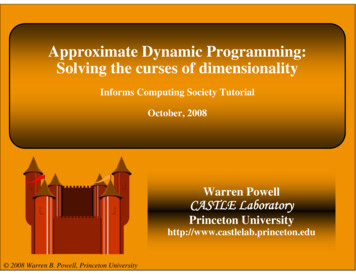
Approximate dynamic es optimal decisions.Mature technologyWeaknessesCannot handle uncertainty.Cannot handle high levelsof complexitySimulationSimulationStrengthsExtremely flexibleHigh level of detailEasily handles uncertaintyWeaknessesModels decisions usinguser-specified rules.Low solution quality.CplexApproximate dynamic programming combines simulation andoptimization in a rigorous yet flexible framework.
Outline A resource allocation modelAn introduction to ADPADP and the post-decision state variableA blood management exampleHierarchical aggregationStepsizesHow well does it work?Some applications»»TransportationEnergy
Blood management Managing blood inventories 2008 Warren B. PowellSlide 64
Blood management Managing blood inventories over timeWeek 0Week 1Week 2Week 3x0S0 S0xx1S1 S1xx2S 2 S 2xx3S3 S3xt 0Rˆ1 , Dˆ1Rˆ 2 , Dˆ 2t 1t 2 2008 Warren B. PowellRˆ3 , Dˆ 3t 3Slide 65
St (Rt,Dˆ tDt , AB AB ,0AB-Dˆ t , AB AB ,1AB ,2A Dˆ t , A AB Rt ,( AB ,0)AB ,0Rt ,( AB ,1)AB ,1Rt ,( AB ,2)AB ,2A-Rt ,( O ,0)O-,0Rt ,(O ,1)O-,1Rt ,( O ,2))ˆRtxDˆ t , AB Dˆ t , AB B B-O-,2O-,0Dˆ t , AB O-,1Dˆ t , AB O-,2O O-AB ,3O-,3Dˆ t , AB Satisfy a demandHold
RtRtxRt 1Rˆt 1, AB Rt ,( AB ,0)AB ,0AB ,0Rt ,( AB ,1)AB ,1AB ,1AB ,1Rt ,( AB ,2)AB ,2AB ,2AB ,2AB ,3AB ,3AB ,0Rt ,( O ,0)O-,0Rt ,(O ,1)O-,1O-,0Rt ,( O ,2)O-,2O-,1O-,1O-,2O-,2O-,3O-,3Dˆ tRˆt 1,O O-,0
RtxRtRt ,( AB ,0)AB ,0AB ,0Rt ,( AB ,1)AB ,1AB ,1Rt ,( AB ,2)AB ,2AB ,2AB ,3Rt ,( O ,0)O-,0Rt ,(O ,1)O-,1O-,0Rt ,( O ,2)O-,2O-,1O-,2O-,3Dˆ t
RtxRtRt ,( AB ,0)AB ,0AB ,0Rt ,( AB ,1)AB ,1AB ,1Rt ,( AB ,2)AB ,2AB ,2AB ,3Rt ,( O ,0)O-,0Rt ,(O ,1)O-,1O-,0Rt ,( O ,2)O-,2O-,1O-,2O-,3Solve this as alinear program.Dˆ tF ( Rt )
Dualsνˆt ,( AB ,0)νˆt ,( AB ,1)νˆt ,( AB ,2)RtxRtAB ,0AB ,0AB ,1AB ,1AB ,2AB ,2AB ,3νˆt ,( AB ,0)O-,0νˆt ,( AB ,1)O-,1O-,0νˆt ,( AB ,2)O-,2O-,1O-,2O-,3Dual variables givevalue additionalunit of blood.Dˆ tF ( Rt )
Updating the value function approximation Estimate the gradient at Rtnνˆtn,( AB ,2)F ( Rt )Rtn,( AB ,2) 2008 Warren B. PowellSlide 71
Updating the value function approximation Update the value function at Rtx ,1nVt n1 1 ( Rtx 1 )νˆtn,( AB ,2)F ( Rt )Rtx ,1nRtn,( AB ,2) 2008 Warre
Introduction to ADP Classical ADP » Most applications of ADP focus on the challenge of handling multidimensional state variables » Start with » Now replace the value function with some sort of approximation tt tt t t t t max ( ,