Transcription
Parallel ComputingChapter 7Performance and ScalabilityJun ZhangDepartment of Computer ScienceUniversity of Kentucky
7.1 Parallel Systems Definition: A parallel system consists of analgorithm and the parallel architecture thatthe algorithm is implemented. Note that an algorithm may have differentperformance on different parallel architecture. For example, an algorithm may performdifferently on a linear array of processors andon a hypercube of processors.
7.2 Performance Metrices for Parallel Systems Run Time: The parallel run time is defined as the timethat elapses from the moment that a parallelcomputation starts to the moment that the lastprocessor finishes execution. Notation: Serial run time TS , parallel run time T P .
7.3 Speedup The speedup is defined as the ratio of the serial runtimeof the best sequential algorithm for solving a problem tothe time taken by the parallel algorithm to solve thesame problem on p processors.TSS TP Example Adding n numbers on an n processorhypercubeT S (n ),T P (log n ),nS (),log n
Using Reduction Algorithm
7.4 Efficiency The efficiency is defined as the ratio of speedup to thenumber of processors. Efficiency measures the fraction oftime for which a processor is usefully utilized.STSE ppT p Example Efficiency of adding n numbers on an n‐processorhypercuben 11E (. ) ()log n nlog n
7.5 Cost The cost of solving a problem on a parallel system is definedas the product of run time and the number of processors. A cost‐optimal parallel system solves a problem with a costproportional to the execution time of the fastest knownsequential algorithm on a single processor. Example Adding n numbers on an n‐processor hypercube.Cost is ( n log n ) for the parallel system and (n ) forsequential algorithm. The system is not cost‐optimal.
7.6 Granularity and Performance Use less than the maximum number of processors. Increase performance by increasing granularity ofcomputation in each processor. Example Adding n numbers cost‐optimally on a hypercube.Use p processors, each holds n/p numbers. First add the n/pnumbers locally. Then the situation becomes adding pnumbers on a p processor hypercube. Parallel run time andcost: ( n / p log p ), ( n p log p )
7.7 Scalability Scalability is a measure of a parallel system’s capacity toincrease speedup in proportion to the number of processors. Example Adding n numbers cost‐optimallyn 2 logpnpS n 2 p logSE pn 2Tp ppnp log pWell‐known Amdahl’s law dictates the achievable speedupand efficiency.
7.8 Amdahl’s Law (1967) The speedup of a program using multiple processors inparallel computing is limited by the time needed for the serialfraction of the problem. If a problem of size W has a serial component Ws, thespeedup of the program isW Ws WspWS (W W s ) / p W sWasS p WsTp
7.9 Amdahl’s Law If Ws 20%, W‐Ws 80%, then10 .8 / p 0 .21 5S as0 .2S p So no matter how many processors are used, the speedupcannot be greater than 5 Amdahl’s Law implies that parallel computing is only usefulwhen the number of processors is small, or when the problemis perfectly parallel, i.e., embarrassingly parallel
7.10 Gustafson’s Law (1988) Also known as the Gustafson‐Barsis’s Law Any sufficiently large problem can be efficiently parallelizedwith a speedupS p ( p 1) where p is the number of processors, and α is the serialportion of the problem Gustafson proposed a fixed time concept which leads toscaled speedup for larger problem sizes. Basically, we use larger systems with more processors to solvelarger problems
7.10 Gustafson’s Law (Cont) Execution time of program on a parallel computer is (a b) a is the sequential time and b is the parallel time Total amount of work to be done in parallel varies linearlywith the number of processors. So b is fixed as p is varied. Thetotal run time is (a p*b) The speedup is (a p*b)/(a b) Define α a/(a b) , the sequential fraction of the executiontime, thenS p ( p 1)
Gustafson’s Law
7.11 Scalability (cont.) Increase number of processors ‐‐ decrease efficiency Increase problem size ‐‐ increase efficiency Can a parallel system keep efficiency by increasing thenumber of processors and the problem sizesimultaneously?Yes: ‐‐ scalable parallel systemNo: ‐‐ non‐scalable parallel systemA scalable parallel system can always be made cost‐optimal byadjusting the number of processors and the problem size.
7.12 Scalability (cont.) E.g. 7.7 Adding n numbers on an n‐processor hypercube, theefficiency is1E ()log n No way to fix E (make the system scalable) Adding n numbers on a p processor hypercube optimally, theefficiency isnE n 2 p log pChoosing n ( p log p ) makes E a constant.
7.13 Isoefficiency Metric of Scalability Degree of scalability: The rate to increase the size of theproblem to maintain efficiency as the number of processorschanges. Problem size: Number of basic computation steps in bestsequential algorithm to solve the problem on a singleprocessor ( W T ).S Overhead function: Part of the parallel system cost(processor‐time product) that is not incurred by the fastestknown serial algorithm on a serial computerTO pT p W
7.14 Isoefficiency FunctionW T O (W , p )TP p1E 1 T O (W , p ) / W Solve the above equation for WW ETO (W , p ) KT O (W , p )1 E The isoefficiency function determines the growth rate of Wrequired to keep the efficiency fixed as p increases. Highly scalable systems have small isoefficiency function.
7.15 Sources of Parallel Overhead Interprocessor communication: increase data locality tominimize communication. Load imbalance: distribution of work (load) is not uniform.Inherent parallelism of the algorithm is not sufficient. Extra computation: modify the best sequential algorithm mayresult in extra computation. Extra computation may be doneto avoid communication.7.6 Minimum Execution TimeTp n 2 log pp
A Few Examples Example Overhead Function for adding n numbers on a pprocessor hypercube.nParallel run time is: T p 2 log ppParallel system cost is: pT p n 2 p log pSerial cost (and problem size) is: TS nThe overhead function is:TO pT p W ( n 2 p log p ) n 2 p log pWhat can we know here?
Example Example Isoefficiency Function for adding n numbers on a pprocessor Hypercube.The overhead function is:TO 2 p log pHence, isoefficiency function isW 2 Kp log pIncreasing the # of processors from p 0 to p1 , the problem size hasto be increased by a factor ofp1 log p1 /( p 0 log p 0 )If p 4 , n 64 , E 0 .8 . If p 16 , for E 0 .8 , we have to have n 512 .
Example Example Isoefficiency Function with a Complex Overhead Function.Suppose overhead function is:TO p 3 / 2 p 3 / 4W 3 / 4For the first term:W Kp 3 / 2For the second term:W Kp 3 / 4W 3 / 4Solving it yieldsW K 4 p3The second term dominates, so the overall asymptotic isoefficiencyfunction is ( p 3 ) .
Example Example Minimum Cost‐Optimal Execution time for Adding nNumbersMinimum execution time is:p n,2T Pmin 2 log nIf, for cost‐optimalW n f ( p ) p log pthenlog n log p log log p log pNow solve (1) for p, we havep f 1( n ) n / log p n / log nT PCost Optimal 3 log n 2 log log n(1)
7.10 Gustafson’s Law (Cont) Execution time of program on a parallel computer is (a b) a is the sequential time and b is the parallel time Total amount of work to be done in parallel varies linearly with the number of processors. So b