Transcription
SPIRiT: Iterative Self-consistent Parallel Imaging Reconstructionfrom Arbitrary k-Space1,2 Michael1Lustig and 2 John M. PaulyDepartment of Electrical Engineering and Computer Science, University of California at Berkeley,Berkeley, California2Magnetic Resonance Systems Research Laboratory, Department of Electrical Engineering, Stan-ford University, Stanford, California.Running head:SPIRiT : Iterative Self-consistent Parallel Imaging ReconstructionAddress correspondence to:Michael Lustig506 Cory HallUniversity of California, BerkeleyBerkeley, CA 94720TEL: (650) 725-57005E-MAIL: mlustig@eecs.berkeley.eduThis work was supported by NIH grants P41RR09784, R01EB007588, R21EB007715 and GE Healthcare.Approximate word count: 126 (Abstract) 6000 (body)Submitted to Magnetic Resonance in Medicine as a Full Paper.
AbstractA new approach to autocalibrating, coil-by-coil parallel imaging reconstruction is presented. It isa generalized reconstruction framework based on self consistency. The reconstruction problem isformulated as an optimization that yields the most consistent solution with the calibration andacquisition data. The approach is general and can accurately reconstruct images from arbitraryk-space sampling patterns. The formulation can flexibly incorporate additional image priors suchas off-resonance correction and regularization terms that appear in compressed sensing. Severaliterative strategies to solve the posed reconstruction problem in both image and k-space domain arepresented. These are based on a projection over convex sets (POCS) and a conjugate gradient (CG)algorithms. Phantom and in-vivo studies demonstrate efficient reconstructions from undersampledCartesian and spiral trajectories. Reconstructions that include off-resonance correction and nonlinear ℓ1 -wavelet regularization are also demonstrated.Key words: Autocalibrating Parallel Imaging, GRAPPA, SENSE, Compressed Sensing,1
IntroductionMultiple receiver coils have been used since the beginning of MRI (1), mostly for the benefit ofincreased signal to noise ratio (SNR). In the late 80’s, Kelton, Magin and Wright proposed in anabstract (2) to use multiple receivers for scan acceleration. However, it was not until the late 90’swhen Sodickson et al. presented their method SMASH (3) and later Pruessmann et al. presentedSENSE (4), that accelerated scans using multiple receivers became a practical and viable option.Multiple receiver coil scans can be accelerated because the data obtained for each coil are acquiredin parallel and each coil image is weighted differently by the spatial sensitivity of its coil. Thissensitivity information in conjunction with gradient encoding reduces the required number of datasamples that is needed for reconstruction. This concept of reduced data acquisition by combinedsensitivity and gradient encoding is widely known as parallel imaging.Over the years, a variety of methods for parallel imaging reconstruction have been developed.These methods differ by the way the sensitivity information is used. Methods like SMASH (3),SENSE (4,5), SPACE-RIP (6), PARS (7) and kSPA (8) explicitly require the coil sensitivities to beknown. In practice, it is very difficult to measure the coil sensitivities with high accuracy. Errorsin the sensitivity are often amplified and even small errors can result in visible artifacts in theimage (9). On the other hand, autocalibrating methods like AUTO-SMASH (10, 11), PILS (12),GRAPPA (13) and APPEAR (14) implicitly use the sensitivity information for reconstruction andavoid some of the difficulties associated with explicit estimation of the sensitivities. Another majordifference is in the reconstruction target. SMASH, SENSE, SPACE-RIP, kSPA and AUTO-SMASHattempt to directly reconstruct a single combined image. Coil-by-coil methods, PILS, PARS andGRAPPA directly reconstruct the individual coil images leaving the choice of combination to theuser. In practice, coil-by-coil methods tend to be more robust to inaccuracies in the sensitivityestimation and often exhibit fewer visible artifacts (9, 14, 15).SENSE is an explicit sensitivity-based, single image reconstruction method. Among all methods, theSENSE approach is the most general. It provides a framework for reconstruction from arbitrary kspace sampling and to easily incorporate additional image priors. When the sensitivities are known,2
SENSE is the optimal solution (14, 15). To the best of the authors’ knowledge, none of the coil-bycoil autocalibrating methods are as flexible and optimal as SENSE. Some proposed methods (16–19)adapt GRAPPA to reconstruct some non-Cartesian trajectories, but these require approximationsand therefore lose some of the ability to remove all the aliasing artifacts.Here, we propose a new approach to parallel imaging reconstruction called SPIRiT. It is a coil-bycoil autocalibrating reconstruction. It is heavily based on the GRAPPA reconstruction, but alsodraws its inspiration from SENSE in the sense that the reconstruction is formulated as an inverseproblem in a very general way. The end result is that the reconstruction is the solution for aleast-squares optimization. SPIRiT is based on self-consistency with the calibration and acquisitiondata. It is flexible and can reconstruct data from arbitrary k-space sampling patterns and easilyincorporates additional image priors. SPIRiT stands for iTerative Self-consistent Parallel ImagingReconstruction.In this paper we first review the foundations of SPIRiT, e.g., the GRAPPA method. We then definethe SPIRiT consistency constraints and show that the reconstruction is a solution to an optimizationproblem. We then extend the method to arbitrary sampling patterns with k-space-based and imagebased approaches. Finally we show that the method can easily introduce additional priors such asoff-resonance correction and regularization.Cartesian GRAPPAThe GRAPPA reconstruction poses the parallel imaging reconstruction as a translation variantinterpolation problem in k-space. It is a self-calibrating coil-by-coil reconstruction method. UnlikeSENSE, which attempts to reconstruct a single combined image, GRAPPA attempts to reconstructthe individual coil images directly.In the traditional GRAPPA (13) algorithm a non-acquired k-space value in the ith coil, at positionr, xi (r), is synthesized by a linear combination of acquired neighboring k-space data from all coils.Let Rr be a set of operators that choose points from a single-coil Cartesian k-space, such that theproduct Rr xi is a vector containing the k-space points in the neighborhood of position r. Let R̃r be3
the operators that choses a smaller subset of only the acquired k-space locations in the neighborhoodof position r. The recovery of xi (r) is given by:xi (r) X grji(R̃r xi ),(1)jwhere grji is a vector set of weights obtained by calibration for the particular sampling pattern is its transpose-conjugate. The full k-space grid is reconstructed byaround position r, and grjisolving Eq. [1] for each un-acquired k-space in all coils and all positions.The linear combination weights, or calibration kernel, used in Eq. [1] are obtained by calibrationfrom a fully acquired k-space region. The calibration finds the set of weights that is the mostconsistent with the calibration data in the least-squares sense. In other words, the calibration stagelooks for a set of weights such that if one tries to synthesize each of the calibration points from theirneighborhood the result should be as close as possible to the true calibration points. More formally,the calibration is described by the following equation:2argmingriXρ CalibX grji(R̃ρ xj ) xi (ρ),(2)jwhere gri is a concatenation of all grji ’s or, gri [gr1i , gr2i , · · · , grN i ]T . The above can be writtenin matrix form as:argmin X̃ gri xi 2 ,(3)griin which the entries of X̃ are all the R̃r xi vectors in the calibration area of k-space that werereordered into a matrix. This equation is often solved as Tykhonov regularized least-squares whichhas the analytic solution:gri (X̃ X̃ βI) 1 X̃ xi .(4)The assumption is that if the calibration consistency holds within the calibration area, it alsoholds in other parts of k-space. Therefore Eq. [1] can be used for the reconstruction. In theoriginal GRAPPA paper, the undersampling pattern was such that the k-space sampling in theneighborhood of the missing points is the same for all points. Therefore a single set of weights4
is enough for reconstruction and the calibration can be performed only once. In 2D accelerationhowever, the sampling pattern around each missing point can be quite different. Different sets ofweights must be obtained for each sampling pattern. As an illustration, consider the 2D GRAPPAreconstruction in Fig. 1a. The figure portrays two equations to solve two missing data points. Eachof the equations uses a different set of calibration weights. The neighborhood size in that examplefor illustration purposes is a square of three k-space pixels.MethodsSPIRiT: a Self Consistency FormulationInspired by GRAPPA, we take on a slightly different approach that has similar properties toGRAPPA, but is more general and uses the data more efficiently. Our aim is to describe thereconstruction as an inverse problem governed by data consistency constraints. The key in theapproach is to separate the consistency constraints into a) consistency with the calibration, and b)consistency with the data acquisition. We formulate these constraints as sets of linear equations.The desired reconstruction is the solution that satisfies the sets of equations best according to asuitable error measure criteria.Even though the acquired k-space data may or may not be Cartesian, ultimately, the desiredreconstruction is a complete Cartesian k-space grid for each of the coils. Therefore, we define theentire Cartesian k-space grid for all the coils as the unknown variables in the equations. Thisstep makes the formulation very general especially when considering noisy data, regularization andnon-Cartesian sampling.Consistency with the CalibrationTraditional GRAPPA enforces calibration consistency only between synthesized points and the acquired points in their associated neighborhoods. The proposed approach expands the notion ofconsistency by enforcing consistency between every point on the grid, xi (r), and its entire neighbor5
hood across all coils (e.g., Rr xj ). It is important to emphasize that the notion, entire neighborhood,includes all the k-space points near xi (r) in all coils whether they were acquired or not. Given theabove, the consistency equation for all k-space positions is given by,xi (r) X gji(Rr xj ).(5)jThe difference between gji here and the traditional GRAPPA weights grji in Eq. [1], is that gjiis a full kernel independent of the actual k-space sampling pattern and is the same for all k-spacepositions. It is obtained by using the operators Rr instead of R̃r in Eq. [2]. Equation [1] definesa large set of decoupled linear equations that can be solved separately. On the other hand, Eq. [5]defines a large set of coupled linear equations. As an illustration, consider Fig. 1b which has asimilar sampling setup as the 2D GRAPPA problem in Fig. 1a. In the figure, three equations areportrayed. It shows that the synthesis of a missing central point depends on both acquired andmissing points in its neighborhood and that the equations are coupled.It is convenient to write the entire coupled system of equations in matrix form. Let x be the entirek-space grid data for all coils, and let G be a matrix containing the gji ’s in the appropriate locations.The system of equations can simply be written as,x Gx.(6)The matrix G is in fact a series of convolution operators (denoted as a b) that convolve the entirek-space with the appropriate calibration kernels,xi Xgij xj .(7)jEquations [6-7] can be explained intuitively. Applying the operation G on x is the same as attempting to synthesize every point from its neighborhood. If x is indeed the correct solution thensynthesizing every point from its neighborhood should yield the exact same k-space data!6
Consistency with the Data AcquisitionOf course, any plausible reconstruction has to be consistent with the real data that were acquiredby the scanner. This constraint can also be expressed as a set of linear equations in matrix form.Let y be the vector of acquired data from all coils (concatenated). Let the operator D be alinear operator that relates the reconstructed Cartesian k-space, x, to the acquired data. The dataacquisition consistency is given byy Dx.(8)This formulation is very general in the sense that x is always Cartesian k-space data, whereas y canbe data acquired with arbitrary k-space sampling patterns. In Cartesian acquisitions, the operatorD selects only acquired k-space locations. The selection can be arbitrary: uniform, variable densityor pseudo random patterns. In non-Cartesian sampling, the operator D represents an interpolationmatrix. It interpolates data from a Cartesian k-space grid onto non-Cartesian k-space locations inwhich the data were acquired.Constrained Optimization FormulationEquations [6] and [8] describe the calibration and data acquisition consistency constraints as sets oflinear equations that the reconstruction must satisfy. However, due to noise and calibration errorsthese equations can only be solved approximately. Therefore, we propose as reconstruction thesolution to an optimization problem given by,minimize (G I)x 2s.t. Dx y 2 ǫ.(9)The parameter ǫ is introduced as a way to control the consistency. It trades off data acquisitionconsistency with calibration consistency. The beauty in this formulation is that the calibrationconsistency is always applied to a Cartesian k-space, even though the acquired data may be nonCartesian. The treatment of non-Cartesian sampling appears only in the data acquisition constraint.This is illustrated more clearly in Fig.
SPIRiT : Iterative Self-consistent Parallel Imaging Reconstruction Address correspondence to: . rji is a vector set of weights obtained by calibration for the particular sampling pattern around position r, and g rji is its transpose-conjugate. The full k-space grid is reconstructed by solving Eq. [1] for each un-acquired k-space in all coils and all positions. The linear combination .