Transcription
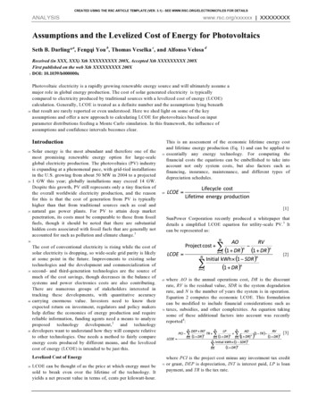
CREATED USING THE RSC ARTICLE TEMPLATE (VER. 3.1) - SEE WWW.RSC.ORG/ELECTRONICFILES FOR DETAILSANALYSISwww.rsc.org/xxxxxx XXXXXXXXAssumptions and the Levelized Cost of Energy for PhotovoltaicsSeth B. Darling*a, Fengqi You b, Thomas Veselka c, and Alfonso Velosa d510Received (in XXX, XXX) Xth XXXXXXXXX 200X, Accepted Xth XXXXXXXXX 200XFirst published on the web Xth XXXXXXXXX 200XDOI: 10.1039/b000000xPhotovoltaic electricity is a rapidly growing renewable energy source and will ultimately assume amajor role in global energy production. The cost of solar generated electricity is typicallycompared to electricity produced by traditional sources with a levelized cost of energy (LCOE)calculation. Generally, LCOE is treated as a definite number and the assumptions lying beneaththat result are rarely reported or even understood. Here we shed light on some of the keyassumptions and offer a new approach to calculating LCOE for photovoltaics based on inputparameter distributions feeding a Monte Carlo simulation. In this framework, the influence ofassumptions and confidence intervals becomes clear.Introduction152025Solar energy is the most abundant and therefore one of themost promising renewable energy option for large-scaleglobal electricity production. The photovoltaics (PV) industryis expanding at a phenomenal pace, with grid-tied installationsin the U.S. growing from about 50 MW in 2004 to a projected1 GW this year; globally installations may exceed 14 GW.Despite this growth, PV still represents only a tiny fraction ofthe overall worldwide electricity production, and the reasonfor this is that the cost of generation from PV is typicallyhigher than that from traditional sources such as coal andnatural gas power plants. For PV to attain deep marketpenetration, its costs must be comparable to those from fossilfuels, though it should be noted that there are substantialhidden costs associated with fossil fuels that are generally notaccounted for such as pollution and climate change.155This is an assessment of the economic lifetime energy costand lifetime energy production (Eq. 1) and can be applied toessentially any energy technology. For computing thefinancial costs the equations can be embellished to take intoaccount not only system costs, but also factors such asfinancing, insurance, maintenance, and different types ofdepreciation schedules.60[1]SunPower Corporation recently produced a whitepaper thatdetails a simplified LCOE equation for utility-scale PV.3 Itcan be represented as:30354045The cost of conventional electricity is rising while the cost ofsolar electricity is dropping, so wide-scale grid parity is likelyat some point in the future. Improvements to existing solartechnologies and the development and commercialization ofsecond- and third-generation technologies are the source ofmuch of the cost savings, though decreases in the balance ofsystems and power electronics costs are also contributing.There are numerous groups of stakeholders interested intracking these developments, with quantitative accuracycarrying enormous value. Investors need to know theirexpected return on investment, regulators and policy makershelp define the economics of energy production and requirereliable information, funding agents need a means to analyzeproposed technology development,2 and technologydevelopers want to understand how they will compete relativeto other technologies. One needs a method to fairly compareenergy costs produced by different means, and the levelizedcost of energy (LCOE) is intended to be just this.[2]6570[3]Levelized Cost of Energy50LCOE can be thought of as the price at which energy must besold to break even over the lifetime of the technology. Ityields a net present value in terms of, cents per kilowatt-hour.This journal is The Royal Society of Chemistry [year]where AO is the annual operations cost, DR is the discountrate, RV is the residual value, SDR is the system degradationrate, and N is the number of years the system is in operation.Equation 2 computes the economic LCOE. This formulationcan be modified to include financial considerations such astaxes, subsidies, and other complexities. An equation takingsome of these additional factors into account was recentlyreported 4:75where PCI is the project cost minus any investment tax creditor grant, DEP is depreciation, INT is interest paid, LP is loanpayment, and TR is the tax rate.Energy and Environmental Science, [year], [vol], 00–00 1
5More importantly, though, one must recognize that each ofthese parameters is associated with a set of assumptions. Inmany cases, there is sufficient uncertainty revolving aroundthese assumptions to render the output only a very crudeestimate. Quantification of that uncertainty is currently absentfrom essentially all LCOE calculations.50Assumptions associated with energy productionSolar Advisor Model101520In an effort to overcome some of the challenges associatedwith performing a reliable LCOE calculation, the NationalRenewable Energy Laboratory, Sandia National Laboratoryand the U.S. Department of Energy have developed a systemperformance model incorporating financing options rangingfrom residential to utility scale named the Solar AdvisorModel (SAM).5 This software is among the most broadly usedto analyze solar technologies for specific locations andprovides users with the capability to probe the relativeinfluence of input parameters on both the energy productionand financial aspects. It represents the best tool publicallyavailable today for the industry to examine the financialfeasibility of a solar project.556065In the SAM analysis, utility-scale LCOE is calculated basedon the required revenues over the project life and is describedas “real” or “nominal” according to:70[4]2575[5]303540where Q n is the electricity generated in year n, R n is therequired revenue from electricity sales in year n, DR real is thereal discount rate (no inflation), and DR nominal is the nominaldiscount rate (with inflation). Hidden within Q and R arenumerous factors such as degradation rate, weather data, priceescalation rate, etc.As with all calculations built around LCOE, however, SAMresults in a specific number and is calculated in such a waythat it inherently incorporates a set of assumptions. (The mostrecent releases of SAM have incorporated the ability toprovide a sensitivity analysis of one or more parametricvariables, which begins to address this issue.) Without adetailed understanding of these underlying assumptions, theirdistribution profiles, and a sensitivity analysis of them, asingle resulting number may give an unfounded confidence inthe certainty of the result.8085909510045In this article, we will shed light on the assumptions that gointo an LCOE calculation for utility-scale PV. When the2 Journal Name, [year], [vol], 00–00dramatic effect of assumptions is revealed, it becomes clearthat a single number from an LCOE calculation does notcapture the uncertainty associated with the economic andfinancial implications of a PV project.Accurately predicting the energy output of a PV system overits lifetime is enormously challenging. It is apparent thatsimply using the vendor’s reported conversion efficiencyunder standard test conditions and the average annual solarinsolation at a given location is dreadfully insufficient. Belowwe describe an improved approach to estimating energyproduction based on input distributions rather than singlenumbers. In each case we outline the rationale behind ourdistributions, which again relies on a series of assumptions.The key is to use the best available data, but more importantlyto understand the source of the data and the uncertaintyassociated with it.In this study we consider a 20 MW utility-scale PV system atthree diverse domestic locations; namely, Sacramento, CA,Chicago, IL, and Boston, MA. Although other types ofsystems are readily analyzed by our model, here wespecifically consider a 1-axis tracking PV system with flatplate collector and an axis tilt equal to the latitute of thelocation. Using the total stated system capacity and anassumed performance of 197 peak watts per square meter, theeffictive area of this PV system is 103,627 m 2. Based oncurrent cost trends for the year 2012, the total capital cost ofthis system is estimated at 54 million. Subsidies provided bythe federal government represent as much as 30% of the totalinstallation cost. The annual insurance cost, which isconservatively assumed to be 0.5% of the installation cost,equals 270,000. In this analysis, we assume a 2.5% inflationrate, 30% federal tax rate, and 8% state tax rate. A 30-yearproject lifetime is considered in this analysis. Evenconsidering only these initial parameters, it becomes clearhow many assumptions go into such a calculation.Solar insolationAs the modeled PV system will be operating beginning today,we use the time series method to forecast the annual solarinsolation in the coming 30 years based on the historialmontly solar insolation data (1960–1990) of the three cities.As the annual solar insolation is nonseasonal, we use fourtime series methods (single moving average, double movingaverage, single exponential smooth, and double exponentialsmooth) for the data set of each city and select the one withthe best forecast as defined by the one having the minimummean square error with respect to the historical data. It turnsout that the single moving average provides the best forecastfor Boston and Sacramento, whereas a single exponentialsmooth works best for the forecast of Chicago. The initialforecasted annual solar insolations of the three cities arepresented in Figure 1. The projections are assumed to follow anormal distribution, which is actually somewhat broader thanthe historical data due to the small sample size. As one looksThis journal is The Royal Society of Chemistry [year]
further into the future with the forecast, the outyears in thetrend toward greater uncertainty, as would be expected.505as temperature, partial shadowing from clouds or debris, andso on. Using a distribution of values takes a step towardcapturing these uncertainties, though even greater accuracy issurely achievable.System degradation rate55106065The rate at which solar cell performance degrades may dependon the type of solar cell, quality of manufacturing, powerproduction level, and local weather/climate. As with theprevious parameters, system degradation rate is generallytreated as a single value in LCOE calculations despite the factthat it is known that even within a single PV installationindividual panels will degrade with substantially differentrates. In this analysis, we assume the system degradation ratehas the probability distribution shown in Figure 3, whichaccounts for a small number of unusually poor performers asis often observed in real systems.15702075Fig. 1 Time series forecasted probability distributions of solar insolationin (a) Boston, (b) Chicago, and (c) Sacramento.Fig. 3 Probability distribution of system degradation rate used in thismodel.Power conversion efficiency25The power conversion efficiency can be affected by manyfactors. In this analysis, we assume it follows a normaldistribution with a mean of 16% and a standard deviation of1% (see Figure 2).30Other production assumptions8085Assumptions associated with costs35Fig. 2 Probability distribution of power conversion efficiency used for thePV system in this model.4045Most analyses of LCOE treat conversion efficiency as aconstant using the value reported by the module vendor usingstandard conditions of illumination and temperature. Inreality, this value only provides an approximation of theactual performance in the real world. Overall efficiencyactually has many parameters rolled up in it. For example, notonly will a PV panel produce less power when there is lesssunlight, in many cases it will also do so less efficiently.Moreover, the dependence of efficiency on insolation is notnecessarily linear. Ideally, one would use real illuminationdependent performance data time synched with forecastedinsolation. Other factors can also affect actual efficiency suchThis journal is The Royal Society of Chemistry [year]In this analysis, we are making a number of additionalassumptions regarding electricity production. (Note that gridintegration costs are yet another factor that can beincorporated into an LCOE calculation, and that distributedpower systems will have a markedly different behavior thancentralized systems.) A few of these include (1) the fact thatconversion efficiency and solar insolation are independentparameters (not actually the case) and (2) weather patternsover the past 30 years provide a reasonable foundation forforecasting sunlight over the next 30 years.9095The two core pieces of an LCOE calculation are energyproduction and cost. There are fundamental assumptionsassociated with each of these, and below we outline some ofthe considerations that enter into the costs. Again, we will useinput distributions to quantitatively capture the uncertaintiesassociated with some of these assumptions.Real discount rate100In addition to risks assocaited with solar insolation levels andthe preformance of PV technologies at a specific location,there is also financial uncertainty in terms of the time value ofmoney. On the down-side, borrowing money now isdisadvantagous if one locks into an interest rate that in thefuture falls percipitously relative to inflation. On the otherEnergy and Environmental Science, [year], [vol], 00–00 3
510hand, if future lending rates increase significantly faster thaninflation, the apperant cost of borrowing may be significantlyless expensive than anticipated at the time of the load. Thisuncertainity is characterized in Figure 4. The shape of thecurve is based on projections made by the Financial ForecastCenter (http://www.forecasts.org/ffund.htm) for the FedFunds interest rate. The general shape was then scaled suchthat the most probable real discount rate reflects currrent ratesfor borrowing money for constructing new PV projects. In theLCOE calculation described below, the real discount rate isconverted to a nominal discount rate using the assumedinflation factor.60Tax rates and subsidies657015into our calculation, but these systems can have a dramaticeffect on comparative fincancial LCOE by either raising thecost of competing technologies based on fossil fuels or byadding value to renewable energy production. Furthermore,incorporating carbon taxes or emission trading will introduceyet another uncertainty that must be properly accounted.As with inputs such as solar insolation, taxes and incentivesfor promoting solar energy also vary widely by location. Inour model we have used a consistent federal tax rate of 30%and state tax rate of 8%. Future policy changes regarding solarsubsidies is yet another uncertainty that is not quantified inthis paper. However, it can greatly influence project financialviablity. For the United States, there is a valuable onlinedatabase that compiles the various state, local, utility, andfederal incentives and policies. 6Analysis of the influence of assumptions20Fig. 4 Probability distribution of the real discount rate used in this model.75Operations and maintenance2530Upkeep of a utility-scale PV system will vary widelydepending on the local conditions. For example, in dustyregions or regions with substantial snowfall, panels will haveto be cleaned more frequently. This cost can shift from year toyear depending on the weather and other factors. We assumethat fixed O&M costs may vary from 8/kW/yr to 20/kW/yr,with the most likely case being approximately 10/kW/year.Therefore, here we assign a triangular distribution to thisparameter, as depicted in Figure 5. Lacking good local data,this distribution is used for all three modeled locations,though it will certainly vary for different environments.35859040458095Fig. 5 Probability distribution of O&M costs used in this model100Carbon market or tax5055Emissions trading (“cap and trade”) is an approach tocontrolling pollution via economic incentives. Market forcesare enlisted to achieve reductions of carbon emissions bycapping the total permissible amount, allocating carboncredits to firms, and enabling the trading of permits. TheEuropean Union has put a greenhouse gas trading scheme intoplace. A carbon tax is an alternative maket-based approachthat directly taxes emissions and thereby provides an incentiveto reduce pollution. As neither system has yet beenimplemented in the United States, we have not included them4 Journal Name, [year], [vol], 00–00105110As any solar LCOE calculation must be performed for aspecific location due to local conditions, we selected threegeographically dispersed locations in the United States:Sacramento, CA, Chicago, IL, and Boston, MA. While thereare other factors that vary between locations, we have takenthe assumption that only solar insolation will be differentbetween these three cities. Surely this overlooks importantfactors such a increased module degradation in regions withgreater temperature and humidity fluctuations, different O&Mcosts (e.g., snowfall amounts in Chicago and Boston ascompared to Sacramento) and non-linearities betweeninsolation and conversion efficiency. Time series forecastingusing three decades of historical insolation at these locationsprovides an estimation of the expected sunlight conditionsover the lifetime of the modeled PV system.To calculate the LCOE for each of these locations (using Eq.3), we have used the parameter probability distributionsoutlined above in a Monte Carlo simulation. This approachprovides a more complete projection of the expected LCOEthan can be offered by a simple calculation using singularinputs.Monte Carlo simulation is a computational mathematicaltechnique that allows one to account for risk in quantitativeanalysis and decision making. Monte Carlo simulationperforms uncertainty analysis by building models of possibleresults through the substitution of a range of values—aprobability distribution—for any factor that has inherentuncertainty. By using probability distributions, variables canhave different probabilities of different outcomes occurring.Probability distributions are an informative method fordescribing uncertainty. During a Monte Carlo simulation,values are sampled at random from the input probabilitydistributions. Each set of samples is called an iteration, andthe resulting outcome from that sample is recorded.Depending upon the number of uncertainties and the rangesspecified for them, a Monte Carlo simulation could involvethousands or millions of iterations. The resulting range of allThis journal is The Royal Society of Chemistry [year]
5calculation results form a distribution from which uncertaintyinformation can be derived with basic statistical methods. Inthis way, Monte Carlo simulation provides a much morecomprehensive view of what may happen. It tells you not onlywhat could happen, but also how likely it is to happen.Monte Carlo simulation provides a number of advantages overdeterministic, or “single-point estimate” analysis:101.2.153.20253035Probabilistic results: Results show not only what couldhappen, but also how likely each outcome is.Sensitivity analysis: With just a few cases, deterministicanalysis makes it difficult to see which variables impactthe outcome the most. In Monte Carlo simulation, it iseasy to see which inputs had the biggest effect onbottom-line results.Correlation of inputs. In Monte Carlo simulation, it ispossible to model interdependent relationships betweeninput variables. It is important for accuracy to representhow, in reality, when some factors goes up, others go upor down accordingly. (Here we have assumedindependent inputs for simplicity.)In this work, we use 1,000,000 iterations for theanlaysis of LCOE for each of the three cities.Carlo simulations produce not only thedistribution of the LCOE, but al
Solar Advisor Model In an effort to overcome some of the challenges associated with performing a reliable LCOE calculation, the National 10 Renewable Energy Laboratory, Sandia National Laboratory and the U.S. Department of Energy hav