WIXLIB

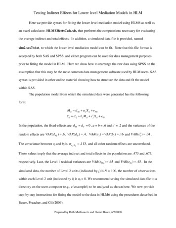
Testing Indirect Effects for Lower level Mediation Models in HLMHere we provide syntax for fitting the lower-level mediation model using HLM6 as well asan excel calculator, HLMEffectsCalc.xls, that performs the computations necessary for evaluatingthe average indirect and total effects. In addition, a simulated data file is provided, namedsim2.sas7bdat, to which the lower level mediation model can be fit. Note that this file format isaccepted by both SAS and SPSS, and either program can be used for data management purposesprior to fitting the model in HLM. Here we show how to rearrange the raw data using SPSS on theassumption that this may be the most common data management software used by HLM users. SASsyntax is provided in other online material showing how to structure the data and fit the modelwithin SAS.The population model from which the simulated data were generated has the followingform:M ijYijd Mja j X ijdYj b j M ijIn the population, the fixed-effects are d MdYeMijc j X ijeYij0 , a b .6 and c' .2 and the variances of therandom effects are VAR (d Mj ) .6 , VAR (dYj ) .4 , VAR (a j ) VAR (b j ) .16 and VAR (c j ) .04 .The covariance between aj and bj isa j ,b j.113 , and all other random effects are uncorrelated.These values imply that the average indirect and total effects in the population are .473 and .673,respectively. Last, the Level 1 residual variances are VAR (eMij ) .65 and VAR(eYij ) .45 . In thesimulated data, the number of Level 2 units (indicated by j) is N 100, the number of observationswithin each Level 2 unit (indicated by i) is nj 8. We recommend saving the simulated data file to adirectory on the users computer (e.g., c:\example\) to be analyzed as shown here. We now providestep-by step instructions for fitting the model to the data in HLM6 using the procedures described inBauer, Preacher, and Gil (2006).Prepared by Ruth Mathiowetz and Daniel Bauer, 6/2/2008

Testing Indirect Effects for Lower level Mediation Models in HLMRestructuring Data in SPSSThe data must first be prepared for the analysis through the creation of a single dependentvariable (Z) from the values of the mediator (M) and the distal outcome (Y). Two selectionvariables are also created, labeled Sy and Sm, to indicate when Z represents M versus Y. A level-2variable (W) is also included in the rearranged data, although the present model does not includethis variable as a predictor of either Y or M. This rearrangement of the data is shown visually inTable 1 of Bauer, Preacher, and Gil (2006). The SPSS syntax for restructuring the data is:*Creating Md variable to use in data restructuring.COMPUTE Md m .EXECUTE .*Restructuring data for multilevel analysis.VARSTOCASES /ID obs/MAKE Z FROM Md y/INDEX Index1(Z)/KEEP m x w id.EXECUTE .The first part of the syntax generates Md as the dependent M variable to be used to construct thesingle dependent variable (Z). Although Md is redundant with M, this redundancy allows for thecreation of Z from Y and M (now Md) and the retention of M as a predictor of Y within Z. TheVARSTOCASES statement begins the data restructuring, with /ID obs creating a variable (obs) toidentify the row at which the observations were located in the original data file. The /MAKE Z FROMMd y statement creates the single dependent variable (Z) by stacking the values of the dependentmediator (Md) and the distal outcome (Y) so each measurement appears on a separate row. Thestatement /INDEX Index1(Z) creates a variable (Index1) to distinguish Y from M values. The/KEEP m x w id statement indicates which variables should be kept as fixed variables, any variablesthat should appear in each row for a given ID value. Our level-2 variable (W) is an example of aPrepared by Ruth Mathiowetz and Daniel Bauer, 6/2/2008

Testing Indirect Effects for Lower level Mediation Models in HLMvariable that should appear as the same value for a given ID value. The following page includesvisual representations of the data set with the Md variable and the restructured data set.First 12 observations of the data set with the Md variable:Restructured data:Prepared by Ruth Mathiowetz and Daniel Bauer, 6/2/2008

Testing Indirect Effects for Lower level Mediation Models in HLMThe following syntax creates the two selection variables labeled Sy and Sm, to indicate when Zrepresents M versus Y:*Creating Sy indicator variable.RECODEIndex1('Md' 0) ('y' 1) INTO Sy .VARIABLE LABELS Sy 'Sy'.EXECUTE .*Creating Sm indicator variable.RECODEIndex1('Md' 1) ('y' 0) INTO Sm .VARIABLE LABELS Sm 'Sm'.EXECUTE .The following syntax creates the level-1 product variables SMX, SYX, and SYM, as well as thelevel-2 product variables SYW and SMW:*Computing variables for analysis.COMPUTE SmX Sm * X .COMPUTE SyX Sy * X .COMPUTE SyM Sy * M .COMPUTE SyW Sy * w .COMPUTE SmW Sm * w .EXECUTE .This data file will serve as both the level 1 and level 2 data file for HLM (it is not necessary tocreate separate level 1 and level 2 data files). The final data set should look like this:Prepared by Ruth Mathiowetz and Daniel Bauer, 6/2/2008

Testing Indirect Effects for Lower level Mediation Models in HLMCreating a MDM file from a SPSS fileAfter launching HLM, select File Make new MDM file Stat package input:Select HLM2, which will bring up this screen:Begin by naming the MDM file (1), then identify the Level-1 (2) and Level 2 (3) data files. Thesewill both be the same data file that was created within SPSS. The choice of „persons within groups‟or „measures within persons‟ is not important for our example; both will fit the same model, theonly difference is the notation HLM uses to display the model.Prepared by Ruth Mathiowetz and Daniel Bauer, 6/2/2008

Testing Indirect Effects for Lower level Mediation Models in HLMNext click on Choose Variables under “Level-1 Specification” to select Level-1 variables foranalysis. For our analysis the single dependent variable Z, the selection variables SY and SM, aswell as the product variables SMX, SYX, and SYM are included as Level-1 variables. The groupingvariable, in our analysis ID, is chosen as the ID variable.Next click on Choose Variables under “Level-2 Specification” to select Level-2 variables foranalysis. For our analysis the grouping variable ID, is chosen as the ID variable and the productvariables SYW, and SMW are included as Level-2 variables. We will not include the Level-2variables in our example model, but one could include such variables, for instance when wishing tocontrol for level 2 covariates, or when evaluating moderated mediation (as in the empirical examplein Bauer, Preacher & Gil, 2006). The effect of SYW would represent the effect of W on Y,whereas the effect of SMW would represent the effect of M on Y.Prepared by Ruth Mathiowetz and Daniel Bauer, 6/2/2008

Testing Indirect Effects for Lower level Mediation Models in HLMAfter the Level 1 and 2 variables have been specified, you can save the MDM template file byclicking Save mdmt file. Next select Make MDM(1). This produces the HLM data file and flashesup some summary statistics for the level 1 and level 2 variables. You can access these again byclicking on Check Stats (2).To start building the model click on Check Stats (2). then Done(3).Prepared by Ruth Mathiowetz and Daniel Bauer, 6/2/2008

Testing Indirect Effects for Lower level Mediation Models in HLMBuilding the modelThe model of interest (equivalent the two equations shown in the first paragraph) is given by thesingle equation:ZijdMj SMija j (SMij X ij ) dYj SYijbj (SYij M ij ) c j (SYij X ij ) eZijWe begin the construction of this model in HLM by selecting Z as the outcome variable:Next select the two selection variables (SY and SM), and the product variables (SMX, SYX andSYM) as the Level 1 variables:Prepared by Ruth Mathiowetz and Daniel Bauer, 6/2/2008

Testing Indirect Effects for Lower level Mediation Models in HLMUnlike most HLM models this model does not have an intercept. Remove the intercept by clickingon INTRCPT1 Delete variable from model:To allow the coefficients to have random effects (representing differences across Level-2 units,select Level-2 and add random components to all Level 1 variables by clicking on all the uvariables:Prepared by Ruth Mathiowetz and Daniel Bauer, 6/2/2008

Testing Indirect Effects for Lower level Mediation Models in HLMAfter the fixed and random effects are specified the estimation settings need to be modified in orderto obtain estimates for the heterogeneous σ² values for SY and SM(i.e., different residual variancesfor the two outcomes). To change these settings select Other Settings Estimation Settings:Select Full maximum likelihood then click on Heterogeneous sigma 2:Prepared by Ruth Mathiowetz and Daniel Bauer, 6/2/2008

Testing Indirect Effects for Lower level Mediation Models in HLMThis window should appear:Select SM as a predictor of Level-1 variance by double-clicking, then select OKThe final model should look like this:Prepared by Ruth Mathiowetz and Daniel Bauer, 6/2/2008

Testing Indirect Effects for Lower level Mediation Models in HLMThe specification of:Allows for the estimation of heterogeneous σ² values for SY and SM, such that the level 1 residualvariance of SY is obtained by eand the level 1 residual variance of SM is e.Lastly, the asymptotic covariance matrices of the fixed effect and variance component estimatesneed to be requested. These values are required for the computation of the standard errors of theaverage indirect and total effects. To obtain these values select Other Settings Output Settings:This window should appear:Select Print variance-covariance matrices, then select OK.Now that the model, estimation and output settings have been specified select Run Analysis to fitthe model to the data.Prepared by Ruth Mathiowetz and Daniel Bauer, 6/2/2008

Testing Indirect Effects for Lower level Mediation Models in HLMHLM Model OutputAn illustration of how the final HLM model is related to the model of interest:The estimates for the fixed and random effects can be found in both the HLM output and the datafiles gamvc.dat and tauvc.dat. Fixed effects in the HLM output:Covariance estimates in the HLM output:The estimates for α0 and α1 in the HLM output:Thus for our example, the estimated residual variance is e-0.67489 .508965 for SY ande-0.67489 0.23976 .646731 for SMPrepared by Ruth Mathiowetz and Daniel Bauer, 6/2/2008

Testing Indirect Effects for Lower level Mediation Models in HLMAt the end of the HLM output there should be a note indicating the creation of 3 data files:By default, these files are placed into the same directory as the program file used to fit the model.Calculating Random Indirect and Total Effects:To calculate the indirect and total effects begin by open the gamvc.dat output file from HLM andthe excel effects calculator spreadsheet HLMEffectsCalc.xls. The first row of gamvc.dat providesthe fixed effects estimates for the level 1 coefficients in the order that they were specified in themodel.The second and subsequent rows of gamvc.dat represent the estimated sampling variances andcovariances of the fixed effect estimates.The values of interest are the estimated values of γ 30, γ40, and γ50 (which correspond to a, c‟ and b,respectively) and their estimated sampling variances and covariances.Prepared by Ruth Mathiowetz and Daniel Bauer, 6/2/2008

Testing Indirect Effects for Lower level Mediation Models in HLMTo better indicate which values are used in the calculations as well as where the values should beentered into the calculator the values have been highlighted in both the gamvc.dat output file andthe excel calculator.Prepared by Ruth Mathiowetz and Daniel Bauer, 6/2/2008