Transcription
3Introductory Guide to HLMWith HLM 7 SoftwareG. David GarsonHLM software has been one of the leading statistical packages for hierarchical linear modeling due to the pioneering work of Stephen Raudenbushand Anthony Bryk, who created the software and authored the leading texton hierarchical linear and nonlinear modeling (Bryk & Raudenbush, 1992;Raudenbush & Bryk, 2002). Though differences among software packages’ capabilities have diminished over time, HLM 7 offers a number of appealing advantages and capabilities. Among these are what many consider to be a more intuitivemodel specification environment, greater ease in creating three- and four-levelmodels, its wide choice of estimation options, integrated likelihood ratio hypothesis testing, graphics options, and the ability easily to handle heterogeneoushierarchical linear models (where the dependent is thought to have different errorvariances for different levels of some grouping variable such as Agency).HLM SOFTWAREScientific Software International (SSI) distributes HLM 7. A free student editionof HLM 7 is available.1 The student edition is full-featured, including examples,but is limited in the size and complexity of models (though it will work with allexample files provided with the software). HLM 7 software operates throughseveral modules, each designed for a different type of HLM model, only some ofwhich can be illustrated here due to space constraints:HLM2. For two-level linear and nonlinear models with one dependent variable.HLM3 and HLM4. For three-level and four-level models with one dependent variable.HGLM. For generalized linear models for distributions other than normal and link functions other than identity, handling binary, count, multinomial, and ordinal outcome variables in Bernoulli, binomial, Poisson, multinomial, and ordinal models.55
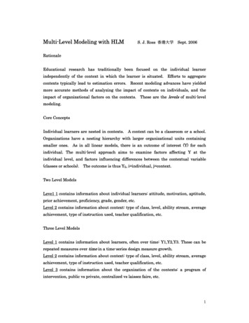
56PA RT I . G U I D EHMLM. For multivariate normal models with more than one outcome variable, including when the level 1 covariance structure is homogenous, heterogeneous, loglinear, orAR(1) (first-order autoregressive).HMLM2. For two-level HMLM models where level 1 is nested within level 2.HCM2. For models where level 1 units are cross-classified by two level 2 units.HCM3. For three-level cross-classified models.HLMHCM. For two- and three-level hierarchical linear models with cross-classifiedrandom effects (ex., repeated test scores nested within students who are cross-classifiedby schools and neighborhoods).In summary, HLM 7 is a versatile and full-featured environment for manylinear and generalized linear mixed models.ENTERING DATA INTO HLM 7HLM software stores data in its own multivariate data matrix (MDM) format,which may be created from raw data or from data files imported from SPSS, SAS,Stata, SYSTAT, or other packages. MDM format files come in flavors keyed tothe several types of HLM modules noted above. File creation options are accessedfrom the HLM File menu, illustrated in Figure 3.1 below. The example belowillustrates data entry from an SPSS .sav file for models of type HLM2, but similarprocedures are followed for other model types.“Stat package input,” depicted above, is the most common method of creating.mdm data files. Further, not only are data commonly prepared using statistical ordata packages outside HLM 7, but as an additional preprocessing step, theresearcher also should rule out multicollinearity among the level 2 (or higher)predictors. Having done this, there are two methods of importing files into HLM 7from other statistical packages.Input Method 1: Separate Files for Each LevelThis method results in faster processing but requires more time to set up thedata. It requires that separate files be created outside of HLM 7 for each level ofHLM analysis. For SPSS, these are .sav files. For SAS, these are SAS 5 transportfiles. Separate SYSTAT and Stata files are also acceptable. For instance, HLM 7software comes with example files from the Singer (1998) “High School andBeyond” study. The SPSS files for this example include HSB1.SAV, which contains the level 2 link field (ID is school ID) and any student-level variables.There are multiple rows per school, one row per student. It is critical that thelevel 1 file is sorted such that all students for a given school ID are adjacent.
CHAPTER 3 . I ntroductory Guide to H L M With H L M 7 S o ftwareFigure 3.1HLM 7 file menuLikewise, the school-level (level 2) file, HSB2.SAV, contains the same level 2link field and any school-level variables.Input Method 2: Using a SingleStatistics Program Data FileThis method2 is easier in terms of data management and is the one illustratedin this chapter. The same statistics package file formats as for Method 1 may beused. For the example, the single data file must be sorted such that all studentsfor a given school ID are adjacent.Making the MDM FileThe next step is to create the .mdm file, which is HLM software’s native dataformat. After it is created, the input data files are not needed. After creating the57
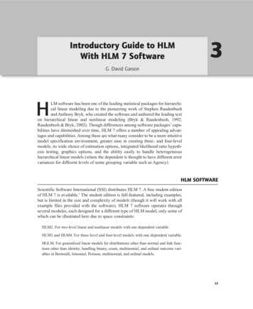
58PA RT I . G U I D EFigure 3.2HLM 7 select MDM type windowinput data file in SPSS, SAS, or another package, HLM 7 is run and “Stat package input” is selected. This causes the “Select MDM type” window illustratedabove to appear.The researcher chooses the HLM model type wanted. For instance, for a simpletwo-level hierarchical linear model, the selection would be HLM2.After selecting HLM2, the “Make MDM - HLM2” dialog box appears, illustrated in Figure 3.3.Here, the following steps are necessary:Set the “Input File Type” to “SPSS/Windows” (or another statistical package format).In the level 1 specification area, click the “Browse” button and browse to the input filefor level 1. Then, as illustrated at the top of Figure 3.4, click the “Choose variables”button, click the checkbox indicating the level 2 link variable (id in the example), andclick the checkboxes of any other level 1 variables in the analysis.In the level 2 specification area, click the “Browse” button and browse to the inputfile for level 2. This may be the same file as for level 1 (following Method 2 above).Again click the “Choose variables” button, click the checkbox indicating the level 2link variable (agency), and click the checkboxes of any other level 2 variables in theanalysis, as indicated in the lower half of Figure 3.4.
CHAPTER 3 . I ntroductory Guide to H L M With H L M 7 S o ftwareFigure 3.3Make MDM - HLM 2 window in HLM 7Save the MDM template file by clicking the “Save mdmt file” button, making sure thefile location window points to the desired folder and giving a filename (add the .mdmtextension), then clicking the “Save” button.To complete the process, the researcher clicks the “Make MDM” button, giving afilename (here, M3 L2.mdm, standing for mixed linear model Chapter 3, 2-level).The .mdm file is created, and the descriptive statistics module runs. Alternatively,one may click the “Check Stats” button. This output, shown in Figure 3.5, shouldbe examined to verify the results. For instance, it is prudent to examine the reportedsample size, which, if low, flags that the researcher has not sorted the Level 1 fileto assure that individual rows for the same level 2 ID (AGENCY in this example)are adjacent.59
60PA RT I . G U I D EFigure 3.4Choose variables windows in HLM 7
CHAPTER 3 . I ntroductory Guide to H L M With H L M 7 S o ftwareFigure 3.561“Check Stats” button output in HLM 7Click the “Done” button to exit to the WHLM model construction screen discussedbelow. At this point, the researcher will have saved three files to the disk: the newlycreated HLM-compatible data file, H3 L2.mdm in this example; the default template creatmdm.mdmt (the researcher may override the default name); and the outputfile above, HLM2MDM.STS (if desired, use File, Save As, to save output under adifferent name, as this default file may get reused with new content if there are multiple runs).THE NULL MODEL IN HLM 7After data are entered, the next step is to create the model. Typically, the firstmodel created is the null model. The null model serves two purposes: (1) It is thebasis for calculating the intraclass correlation coefficient (ICC), which is the usualtest of whether multilevel modeling is needed; and (2) it outputs the deviancestatistic (-2LL) and other coefficients used as a baseline for comparing later, morecomplex models. For the current example, the null model addresses the question,“Is there a (level 2) agency effect on the (level 1) intercept of performance score,which represents the mean score?” If there is an agency effect, then ordinaryregression methods will suffer from correlated error, and some form of linearmixed modeling is required.The null model, like all two-level hierarchical models in HLM 7, is created inthe WHLM modeling dialog, illustrated in Figure 3.6. This dialog is reachedeither on clicking “Done” in the “MAKE MDM” dialog or, if the MDM file was
62Figure 3.6PA RT I . G U I D EWHLM modeling window in HLM 7: Null modelpreviously saved, from the HLM menu by selecting File, “Create a new modelusing an existing MDM file,” and then opening the appropriate .mdm file.In the WHLM modeling dialog illustrated in Figure 3.6, the employee level(level 1) dependent variable performance score (SCORE0) is designated as the outcome variable. No other predictors are added. HLM 7 already knows “Agency” isthe level 2 grouping variable and automatically assumesit is a predictor of the level 1 intercept of SCORE0.Table 3.1 Summary of the Null ModelWhen SCORE0 is designated as the outcome variable, HLM 7 constructs and displays the model, in thiscase the null model (also called the intercept-only modelLevel 1 Modelor the one-way ANOVA model with random effects).SCORE0ij β0j rijThe null model is shown in Table 3.1 below. Clickingthe “Mixed” button at the bottom of the WHLM dialogLevel 2 Modelcreates the combined HLM equation shown at the botβ0j γ00 u0jtom of the figure: The two separate equations shown inMixed Modelthe upper main window are mathematically equivalentto the single combined mixed model equation. ForSCORE0ij γ00 u0j rijlearning purposes, it is easier to examine the equations
CHAPTER 3 . I ntroductory Guide to H L M With H L M 7 S o ftwareat each level. At level 1, SCORE0 is predicted by an intercept term and a randomterm. The symbol for the intercept term varies depending on the distributionspecified for the outcome variable (this is done in the “Basic Settings” window,described below) and is expressed equivalently but differently in output.The level 1 intercept term, expressed as β0j in output, is a function of a randomintercept term at level 2 (γ00) and a level 1 residual error term (rij). The level 1intercept, in turn, is a function of the grand mean (γ00) across level 2 units, whichare agencies in this example, plus a random error term (u0j), signifying the intercept is modeled as a random effect. Substituting the right-hand side of the level 2equation into the level 1 equation gives the mixed model equation for the nullrandom intercept model. HLM 7 will create one level 1 regression for eachagency, and then will utilize the variance in these intercepts when estimatingparameters and standard errors at level 1. This is what makes the process differentfrom ordinary regression, where a single overall intercept is estimated.Before calculating estimates, the researcher may specify the distribution of theoutcome variable by selecting “Basic Settings” from the main menu bar, yieldingthe window shown in Figure 3.7. The normal distribution, used in this example, isthe default. Other available specifications support Bernoulli, Poisson, multinomial,and ordinal distributions. Selecting “Bernoulli” for a binary outcome variableapplies a logistic link function, and in the ensuing multilevel logistic regression,interpretations are in terms of the log odds of the outcome rather than in terms ofthe raw outcome itself. Selecting “Multinomial” creates a multilevel multinomialregression using a logit link. “Ordinal” supports multilevel ordinal regression models. Multilevel Poisson regression models employ a Poisson log link and require anexposure variable (time, for example). In this window, one may also specify thename and location of the output statistics file and the output graphics file.It is also possible to modify model estimation settings prior to running themodel by selecting “Other Settings” from the main menu bar, then “EstimationSettings,” as illustrated in Figure 3.8. Estimation settings were discussed inChapter 2. For the null model, we use the default setting, restricted maximumlikelihood estimation. There is also an “Iterations Settings” window, also fromthe “Other Settings” menu. Though not illustrated here, it provides options discussed in Chapter 2 with regard to estimation settings.One may also select “Other Settings” from the main menu bar, then “OutputSettings” to obtain the window shown in Figure 3.9. For this model, one maychoose to print out variance–covariance matrices or to restrict output to the mainresults. The default is restricted output and no matrices.To run the null model, the researcher simply selects “Run Analysis” from themain menu bar. Output is sent to the file location and a name is specified in the“Basic Model Specifications” window (Figure 3.7). To view the output, selectFile, View Output, from the main menu bar. For this example, the critical outputof the null model looks as shown in Table 3.2.The phrase “Number of estimated parameters 2” refers to the fact that in a nullmodel, estimates are made for the level 1 intercept and the level 2 intercept. In the63
64PA RT I . G U I D EFigure 3.7Basic Model Specifications window from Basic Settings menu in HLM 7final variance components table, the fact that the component for the intercept(161.94, which HLM labels tau, τ) is significant means that the intercept of theoutcome variable, SCORE0, is significantly affected by its predictors, which inthis example is the level 2 effect of agency. A non-significant intercept in the variance components table term (not the case here) would mean that after other variables in the model are controlled, there would be no residual between-groupsvariance in the level 1 dependent variable (Score0). The agency effect is smallerthan the residual variance component (212.69, which HLM also labels sigmasquared, σ2), indicating that there is still considerable residual variation in Score0yet to be explained and that a model with additional predictors may be needed.The fact that the intercept component is significant means that the intraclasscorrelation coefficient, ICC, is also significant, indicating that a multilevel modelis appropriate and needed. ICC varies from 1.0 when group means differ butwithin any group there is no variation, to - 1/(n - 1) when group means are allthe same but within-group variation is very large. At the extreme, when ICC
65CHAPTER 3 . I ntroductory Guide to H L M With H L M 7 S o ftwareFigure 3.8Estimation Settings window from Other Settings menu in HLM 7Figure 3.9Output Settings window for HLM2Table 3.2Final Estimation of Variance Components for the Two-Level Null ModelRandom effectStandard deviationVariance componentd.f.χ2p-valueINTRCPT1, u012.72558161.940291312391.61810 0.001level-1, r14.58375212.68575Statistics for current covariance components modelDeviance 29028.420032Number of estimated parameters 2
66PA RT I . G U I D Eapproaches 0 or is negative, hierarchical modeling is not appropriate. For thisexample, the magnitude of ICC may be calculated as the intercept variance component in the null model divided by the total of variance components. That is,ICC 161.94/(161.94 212.69) .43.The fixed effect tables are of lesser interest in a null model but are presentedin Table 3.3. Mean performance score (the intercept at level 1) is estimated to be55.60 for this example, when the level 2 grouping variable, agency, is the onlyeffect modeled. Confidence limits around the mean, of course, are approximatelyplus or minus two standard errors. The lower table, “with robust standard errors,”produces the same estimate but has a slightly different standard error. Robuststandard errors are recommended when it is possible the researcher has specifiedthe wrong distribution of the dependent variable. Significant differences betweenthe ordinary and robust estimates of the standard error may flag a problem with thedistribution specified by the researcher. This is not the case in this example,which specified a normal distribution (which is the default).The “Deviance” value of 29028.42 in Table 3.2 is the basis of model fit measures. While not used at this point, for the null model it is the baseline model fit.More complex models are assessed in part by how greatly they reduce deviance(which is also called -2 log likelihood, -2LL, and model chi-square). These testsof the difference in deviance values between models are likelihood ratio tests,requested in HLM 7 by selecting “Other Settings” from the main menu bar, then“Hypothesis Testing,” as discussed later in this chapter. In summary, at the end ofanalysis of the null model we have demonstrated that there is a significant agencyeffect on employee performance scores; that therefore multilevel modeling isTable 3.3Fixed Effects Tables for the Null ModelFinal estimation of fixed effectsFixed effectCoefficientStandard 524131 0.001For INTRCPT1, β0INTRCPT2, γ00Final estimation of fixed effects (with robust standard errors)Fixed effectCoefficientStandard errort-ratioApprox. d.f.p-value55.5982481.14142348.710131 0.001For INTRCPT1, β0INTRCPT2, γ00
CHAPTER 3 . I ntroductory Guide to H L M With H L M 7 S o ftware67needed; and that additional, more complex models with more predictors shouldreduce significantly the baseline deviance value of 29028.42.A RANDOM COEFFICIENTS REGRESSION MODEL IN HLM 7Given level 1 representing employees, with performance score as an outcome(dependent) variable, and level 2 representing agencies, a random coefficientsregression model is one with one or more level 1 predictors such as gender, yearsof experience, or a binary indicator for whether the employee is certified or not.The level 2 grouping variable (Agency) remains a random factor, but there are noother level 2 predictors. The “coefficients” term in the label means that theagency effect is used not only to model the level 1 intercept of SCORE0 as anoutcome, but also to model the regression coefficients of the level 1 predictors.As an example of random coefficients (RC) regression, employee performancescore (score0) at level 1 is predicted from the level 1 covariates years of experience (YrsExper) and sex (Gender, where 0 male, 1 female). Note that HLM 7enters binary variables like Gender as covariates by default. There are no predictors at level 2, but Agency is the subjects variable under which employees aregrouped. The intercept of score0 at level 1 and the b coefficient of YrsExper atlevel 1 are both modeled as random effects of Agency. Gender is treated as asimple level 1 fixed effect. This model explores whether the Agency effect discovered in the null model may be attributed in part to some agencies having moreexperienced employees than others. The model also explores whether the demographic variable, Gender, modifies the relationship of years of experience toperformance score.Figure 3.10 illustrates this RC regression model. An often-cited advantage ofHLM software is how its user interface clearly separates regression models atdifferent levels. Here, at level 1, score0 is predicted from YrsExper and Gender,plus an intercept term β0j and an error term rij:SCORE0ij β0j β1j*(YRSEXPERij) β2j*(GENDERij) rijAt level 2, there are no predictors. However, the level 1 intercept is predictedby the level 2 mean (γ00) of score0 plus a level 2 error term (u0j). The level 2 erro
In summary, HLM 7 is a versatile and full-featured environment for many linear and generalized linear mixed models. ENTERING DATA INTO HLM 7 HLM software stores data in its own multivariate data matrix (MDM) format, which may be created from raw data or from data files imported from SPSS, SAS, Stata, SYSTAT, or other packages.File Size: 3MB