Transcription
FoMP: Vectors, Tensors and Fields1
Contents1 Vectors1.11.21.31.4Review of Vectors . . . . . . . . . . . . . . . . . . . . . . . . . . . . . . . . .61.1.1Physics Terminology (L1) . . . . . . . . . . . . . . . . . . . . . . . .61.1.2Geometrical Approach . . . . . . . . . . . . . . . . . . . . . . . . . .61.1.3Scalar or dot product . . . . . . . . . . . . . . . . . . . . . . . . . . .71.1.4The vector or ‘cross’ product . . . . . . . . . . . . . . . . . . . . . . .71.1.5The Scalar Triple Product . . . . . . . . . . . . . . . . . . . . . . . .81.1.6The Vector Triple Product . . . . . . . . . . . . . . . . . . . . . . . .91.1.7Some examples in Physics . . . . . . . . . . . . . . . . . . . . . . . .9Equations of Points, Lines and Planes . . . . . . . . . . . . . . . . . . . . . .101.2.1Position vectors (L2) . . . . . . . . . . . . . . . . . . . . . . . . . . .101.2.2The Equation of a Line . . . . . . . . . . . . . . . . . . . . . . . . . .101.2.3The Equation of a Plane . . . . . . . . . . . . . . . . . . . . . . . . .111.2.4Examples of Dealing with Vector Equations . . . . . . . . . . . . . .11Vector Spaces and Orthonormal Bases . . . . . . . . . . . . . . . . . . . . .141.3.1Review of vector spaces (L3) . . . . . . . . . . . . . . . . . . . . . . .141.3.2Linear Independence . . . . . . . . . . . . . . . . . . . . . . . . . . .151.3.3Standard orthonormal basis: Cartesian basis . . . . . . . . . . . . . .161.3.4Suffix or Index notation . . . . . . . . . . . . . . . . . . . . . . . . .16Suffix Notation . . . . . . . . . . . . . . . . . . . . . . . . . . . . . . . . . .181.4.1Free Indices and Summation Indices (L4) . . . . . . . . . . . . . . . .181.4.2Handedness of Basis . . . . . . . . . . . . . . . . . . . . . . . . . . .191.4.3The Vector Product in a right-handed basis . . . . . . . . . . . . . .191.4.4Summary of algebraic approach to vectors . . . . . . . . . . . . . . .201.4.5The Kronecker Delta Symbol δij . . . . . . . . . . . . . . . . . . . .Matrix representation of δij . . . . . . . . . . . . . . . . . . . . . . .2122More About Suffix Notation . . . . . . . . . . . . . . . . . . . . . . . . . . .221.5.1Einstein Summation Convention (L5) . . . . . . . . . . . . . . . . . .221.5.2Levi-Civita Symbol ijk . . . . . . . . . . . . . . . . . . . . . . . . .Vector product . . . . . . . . . . . . . . . . . . . . . . . . . . . . . .231.4.61.561.5.3224
1.5.41.61.7Product of two Levi-Civita symbols . . . . . . . . . . . . . . . . . . .26Change of Basis . . . . . . . . . . . . . . . . . . . . . . . . . . . . . . . . . .271.6.1Linear Transformation of Basis (L6) . . . . . . . . . . . . . . . . . . .271.6.2Inverse Relations . . . . . . . . . . . . . . . . . . . . . . . . . . . . .271.6.3The Transformation Matrix . . . . . . . . . . . . . . . . . . . . . . .281.6.4Examples of Orthogonal Transformations . . . . . . . . . . . . . . . .291.6.5Products of Transformations . . . . . . . . . . . . . . . . . . . . . . .301.6.6Improper Transformations . . . . . . . . . . . . . . . . . . . . . . . .301.6.7Summary . . . . . . . . . . . . . . . . . . . . . . . . . . . . . . . . .31Transformation Properties of Vectors and Scalars . . . . . . . . . . . . . . .311.7.1Transformation of vector components (L7) . . . . . . . . . . . . . . .311.7.2The Transformation of the Scalar Product . . . . . . . . . . . . . . .321.7.3Summary of story so far . . . . . . . . . . . . . . . . . . . . . . . . .332 Tensors2.12.22.32.435Tensors of Second Rank . . . . . . . . . . . . . . . . . . . . . . . . . . . . .352.1.1Nature of Physical Laws (L8) . . . . . . . . . . . . . . . . . . . . . .352.1.2Examples of more complicated laws . . . . . . . . . . . . . . . . . . .362.1.3General properties . . . . . . . . . . . . . . . . . . . . . . . . . . . .382.1.4Invariants . . . . . . . . . . . . . . . . . . . . . . . . . . . . . . . . .382.1.5Eigenvectors . . . . . . . . . . . . . . . . . . . . . . . . . . . . . . . .39The Inertia Tensor . . . . . . . . . . . . . . . . . . . . . . . . . . . . . . . .392.2.1Computing the Inertia Tensor (L9) . . . . . . . . . . . . . . . . . . .392.2.2Two Useful Theorems. . . . . . . . . . . . . . . . . . . . . . . . . .42Eigenvectors of Real, Symmetric Tensors . . . . . . . . . . . . . . . . . . . .432.3.1Construction of the Eigenvectors (L10) . . . . . . . . . . . . . . . . .442.3.2Important Theorem and Proof . . . . . . . . . . . . . . . . . . . . . .452.3.3Degenerate eigenvalues . . . . . . . . . . . . . . . . . . . . . . . . . .47Diagonalisation of a Real, Symmetric Tensor (L11) . . . . . . . . . . . . . .482.4.1Symmetry and Eigenvectors of the Inertia Tensor . . . . . . . . . . .502.4.2Summary . . . . . . . . . . . . . . . . . . . . . . . . . . . . . . . . .523 Fields523
3.13.23.33.4Examples of Fields (L12) . . . . . . . . . . . . . . . . . . . . . . . . . . . . .523.1.1Level Surfaces of a Scalar Field . . . . . . . . . . . . . . . . . . . . .533.1.2Gradient of a Scalar Field . . . . . . . . . . . . . . . . . . . . . . . .543.1.3Interpretation of the gradient . . . . . . . . . . . . . . . . . . . . . .553.1.4Directional Derivative . . . . . . . . . . . . . . . . . . . . . . . . . .56More on Gradient; the Operator ‘Del’ . . . . . . . . . . . . . . . . . . . . . .573.2.1Examples of the Gradient in Physical Laws (L13) . . . . . . . . . . .573.2.2Examples on gradient . . . . . . . . . . . . . . . . . . . . . . . . . . .573.2.3Identities for gradients . . . . . . . . . . . . . . . . . . . . . . . . . .583.2.4Transformation of the gradient. . . . . . . . . . . . . . . . . . . . .603.2.5The Operator ‘Del’ . . . . . . . . . . . . . . . . . . . . . . . . . . . .60More on Vector Operators . . . . . . . . . . . . . . . . . . . . . . . . . . . .613.3.1Divergence (L14) . . . . . . . . . . . . . . . . . . . . . . . . . . . . .623.3.2Curl . . . . . . . . . . . . . . . . . . . . . . . . . . . . . . . . . . . .633.3.3Physical Interpretation of ‘div’ and ‘curl’ . . . . . . . . . . . . . . . .643.3.4The Laplacian Operator 2 . . . . . . . . . . . . . . . . . . . . . . .65Vector Operator Identities . . . . . . . . . . . . . . . . . . . . . . . . . . . .663.4.1Distributive Laws (L15) . . . . . . . . . . . . . . . . . . . . . . . . .663.4.2Product Laws . . . . . . . . . . . . . . . . . . . . . . . . . . . . . . .663.4.3Products of Two Vector Fields . . . . . . . . . . . . . . . . . . . . . .673.4.4Identities involving 2 gradients . . . . . . . . . . . . . . . . . . . . . .683.4.5Polar Co-ordinate Systems . . . . . . . . . . . . . . . . . . . . . . . .694 Integrals over Fields4.14.270Scalar and Vector Integration and Line Integrals . . . . . . . . . . . . . . . .704.1.1Scalar & Vector Integration (L16) . . . . . . . . . . . . . . . . . . . .704.1.2Line Integrals . . . . . . . . . . . . . . . . . . . . . . . . . . . . . . .714.1.3Parametric Representation of a line integral . . . . . . . . . . . . . .72The Scalar Potential (L17) . . . . . . . . . . . . . . . . . . . . . . . . . . . .754.2.1Theorems on Scalar Potentials . . . . . . . . . . . . . . . . . . . . . .754.2.2Finding Scalar Potentials . . . . . . . . . . . . . . . . . . . . . . . . .774.2.3Conservative forces: conservation of energy . . . . . . . . . . . . . . .784
4.2.4Physical Examples of Conservative Forces . . . . . . . . . . . . . . .79Surface Integrals (L18) . . . . . . . . . . . . . . . . . . . . . . . . . . . . . .814.3.1Parametric form of the surface integral . . . . . . . . . . . . . . . . .83More on Surface and Volume Integrals . . . . . . . . . . . . . . . . . . . . .854.4.1The Concept of Flux (L19) . . . . . . . . . . . . . . . . . . . . . . . .854.4.2Other Surface Integrals . . . . . . . . . . . . . . . . . . . . . . . . . .864.4.3Parametric form of Volume Integrals . . . . . . . . . . . . . . . . . .87The Divergence Theorem . . . . . . . . . . . . . . . . . . . . . . . . . . . . .894.5.1Integral Definition of Divergence . . . . . . . . . . . . . . . . . . . . .894.5.2The Divergence Theorem (Gauss’s Theorem) . . . . . . . . . . . . . .904.6The Continuity Equation . . . . . . . . . . . . . . . . . . . . . . . . . . . . .914.7Sources and Sinks . . . . . . . . . . . . . . . . . . . . . . . . . . . . . . . . .924.8Examples of the Divergence Theorem (L21) . . . . . . . . . . . . . . . . . .934.9Line Integral Definition of Curl and Stokes’ Theorem . . . . . . . . . . . . .944.9.1Line Integral Definition of Curl . . . . . . . . . . . . . . . . . . . . .944.9.2Cartesian form of Curl . . . . . . . . . . . . . . . . . . . . . . . . . .954.9.3Stokes’ Theorem . . . . . . . . . . . . . . . . . . . . . . . . . . . . .964.9.4Applications of Stokes’ Theorem (L22) . . . . . . . . . . . . . . . . .984.9.5Example on joint use of Divergence and Stokes’ Theorems . . . . . . 1004.34.44.55
1Vectors1.1Review of Vectors1.1.1Physics TerminologyScalar : quantity specified by a single number;Vector : quantity specified by a number (magnitude) and a direction;e.g. speed is a scalar, velocity is a vector1.1.2Geometrical ApproachA vector is represented by a ‘directed line segment’ with a length and direction proportionalto the magnitude and direction of the vector (in appropriate units). A vector can be considered as a class of equivalent directed line segments e.g.QSAAPBoth displacements from P to Q and from R to S are representedby the same vector. Also, different quantities can be representedby the same vector e.g. a displacement of A cm, or a velocity of Ams 1 or . . . , where A is the magnitude or length of vector ARNotation: Textbooks often denote vectors by boldface: A but here we use underline: ADenote a vector by A and its magnitude by A or A. Always underline a vector to distinguishit from its magnitude . A unit vector is often denoted by a hat  A / A and represents adirection.Addition of vectors—parallelogram lawi.e.A BAA B B A(A B) C A (B C)BMultiplication by scalars,A vector may be multiplied by a scalar to give a new vector e.g.AαA(for α 0)(forα 0)6(commutative) ;(associative) .
Also αA α(A B)α(βA)(α β)A1.1.3 α A αA αB(αβ)AαA βA .(distributive)(associative)Scalar or dot productThe scalar product (also known as the dot product) between two vectors is defined asdef(A · B) AB cos θ, where θ is the angle between A and BB(A · B) is a scalar — i.e. a single number.θA.Notes on scalar product(i) A · B B · A ; A · (B C) A · B A · C(ii) n̂ · A the scalar projection of A onto n̂, where n̂ is a unit vector(iii) (n̂ · A) n̂ the vector projection of A onto n̂(iv) A vector may be resolved with respect to some direction n̂ into a parallel componentAk (n̂ · A)n̂ and a perpendicular component A A Ak . You should check thatA · n̂ 0(v)1.1.4A · A A 2 which defines the magnitude of a vector. For a unit vector  ·  1The vector or ‘cross’ productdef(A B) AB sin θ n̂ , where n̂ in the ‘right-hand screw direction’i.e. n̂ is a unit vector normal to the plane of A and B, in the direction of a right-handedscrew for rotation of A to B (through π radians).7
(AX B)θA.(A B) is a vector — i.e. it has a direction and a length.Bvn[It is also called the cross or wedge product — and in the latter case denoted by A B.]Notes on vector product(i) A B B A(ii) A B 0 if A, B are parallel(iii) A (B C) A B A C(iv) A (αB) αA B1.1.5The Scalar Triple ProductThe scalar triple product is defined as followsdef(A, B, C) A · (B C)Notes(i) If A, B and C are three concurrent edges of a parallelepiped, the volume is (A, B, C).To see this, note that:(BX C)aφvnO.AcθdCBbarea of the base height volume area of parallelogram ObdcB C sin θ B C A cos φ n̂ · Aarea of base heightB C sin θ n̂ · AA · (B C)(ii) If we choose C, A to define the base then a similar calculation gives volume B ·(C A)We deduce the following symmetry/antisymmetry properties:(A, B, C) (B, C, A) (C, A, B) (A, C, B) (B, A, C) (C, B, A)(iii)If A, B and C are coplanar (i.e. all three vectors lie in thesame plane) then V (A, B, C) 0, and vice-versa.8
1.1.6The Vector Triple ProductThere are several ways of combining 3 vectors to form a new vector.e.g. A (B C); (A B) C, etc. Note carefully that brackets are important, sinceA (B C) 6 (A B) C .Expressions involving two (or more) vector products can be simplified by using the identity:–A (B C) B(A · C) C(A · B) .This is a result you must memorise. We will prove it later in the course.1.1.7Some examples in Physics(i) Angular velocityConsider a point in a rigid body rotating with angular velocity ω: ω is the angular speedof rotation measured in radians per second and ω̂ lies along the axis of rotation. Let theposition vector of the point with respect to an origin O on the axis of rotation be r.ωvθ rYou should convince yourself that v ω r by checking that thisgives the right direction for v; that it is perpendicular to the planeof ω and r; that the magnitude v ωr sin θ ω radius of circlein which the point is travellingO(ii) Angular momentumNow consider the angular momentum of the particle defined by L r (mv) where m isthe mass of the particle.Using the above expression for v we obtain L mr (ω r) m ωr 2 r(r · ω)where we have used the identity for the vector triple product. Note that only if r is perpendicular to ω do we obtain L mωr 2 , which means that only then are L and ω in the samedirection. Also note that L 0 if ω and r are parallel.end of lecture 19
1.2Equations of Points, Lines and Planes1.2.1Position vectorsA position vector is a vector bound to some origin and gives the position of a point relativeto that origin. It is often denoted x or r.rThe equation for a point is simply r a where a is some vector.O1.2.2The Equation of a LineSuppose that P lies on a line which passes through a point A which has a position vector awith respect to an origin O. Let P have position vector r relative to O and let b be a vectorthrough th
1.1.4 The vector or ‘cross’ product (A B) def ABsin n ;where n in the ‘right-hand screw direction’ i.e. n is a unit vector normal to the plane of Aand B, in the direction of a right-handed