Transcription
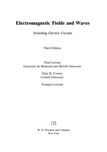
Electromagnetic Fields and WavesIncluding Electric CircuitsThird EditionPaul LorrainUniversite de Montreal and McGill UniversityDale R. CorsonCornell UniversityFran ;ois Lorrainrnw. H. Freeman and CompanyNew York
Cover image: Lines of E and of H in an optical waveguide. See page 668.Back cover image: Differentiating circuit. See page 144.Library of Congress Cataloging-in-Publication DataLorrain, Paul.Electromagnetic fields and waves.Includes index.1. Electromagnetic fields. 2. Electromagnetic waves.I. Corson, Dale R.II. Lorrain, Fran"oisIII. TitleQC665.E4L6786-31803530 . 1 '4 11 987ISBN 0-716-71823-5ISBN 0-716-71869-3 (pbk.)Copyright 1 988 by W. H. Freeman and CompanyNo part of this book may be reproduced by any mechanical,photographic, or electronic process, or in the form of aphonographic recording, nor may it be stored in a retrievalsystem, transmitted, or otherwise copied for public orprivate use without written permission from the publisher.Printed in the United States of America234567890VB65432()HI)
CONTENTS123viiiPrefaceVECTOR OPERATORS29PHASORSELECTRIC FIELDS I42Coulomb's Law and Gauss's Law4ELECTRIC FIELDS II64The Equations of Poisson and Laplace. Charge Conservation.Conductors56ELECTRIC FIELDS III84ELECTRI C FIELDS IV101Electric MultipolesEnergy, Capacitance, and Forces*7ELECTRIC FIELDS V*8ELECTRIC FIELDS VI9ELECTRIC FIELDS VII10ELECTRIC FIELDS VIII119Electric Circuits A : RC Circuits149Electric Circuits B : Circuit Theorems172Dielectric Materials A: Bound Charges and the Electric FluxDensity D192Dielectric Materials B: Real Dielectrics, Continuity Conditions atan Interface, and Stored Energy11ELECTRIC FIELDS IX211Images. Laplace's Equation in Rectangular Coordinates Asterisks mean that the chapters can be skipped without losing continuity.
CONTENTSVI12ELECTRIC FIELDS X225Laplace's Equation in Spherical Coordinates . Poisson's Equationfor E* 13RELATIVITY I238The Lorentz Transformation and Space-time* 14RELA TIVITY II251The Lorentz Contraction and Time Dilation. The Transformationof a Velocity* 15RELATIVITY III265RELATIVITY IV284Mass, Momentum, Force, and Energy*16The Field of a Moving Electric Charge* 17RELATIVITY V308Maxwell's Equations. The Four-Potential A18MAGNETIC FIELDS I326The Magnetic Flux Density B and the Vector Potential A34819MAGNETIC FIELDS II20MAGNETIC FIELDS III360MAGNETIC FIELDS IV374The Vector Potential A . Ampere's Circuital Law*21Magnetic Materials A : The Magnetic Flux Density B and theMagnetic Field Strength HMagnetic Materials B: Ferromagnetism and Magnetic Circuits22MAGNETIC FIELDS V387The Magnetic Forces on Charges and Currents23MAGNETIC FIELDS VIThe Faraday Induction Law*24MAGNETIC FIELDS VII412437Electric Circuits C: Mutual and Self -Inductance*25MAGNETIC FIELDS VIII452Electric Circuits D : Inductive Circuits and Transformers26MAGNETIC FIELDS IX471Magnetic Energy and Macroscopic Magnetic Forces27MAXWELL'S EQUATIONS492
('ONTENTS28VllPLANE ELECTROMAGNETIC WAVES I514Uniform Plane Waves in Free Space, Nonconductors, andConductors*29PLANE ELECTROMAGNETIC WAVES IIWaves in Good Conductors and in Plasmas30536PLANE ELECTROMAGNETIC WAVES III554PLANE ELECTROMAGNETIC WAVES IV578Reflection and Refraction A : The Basic Laws and Fresnel'sEquations31Reflection and Refraction B : Nonuniform Plane Waves and TotalReflection32PLANE ELECTROMAGNETIC WAVES V594Reflection and Refraction C: Reflection and Refraction at theSurface of a Good Conductor33610GUIDED WAVES IGeneral Principles. The Coaxial and Microstrip Lines34GUIDED WAVES II626The Hollow Rectangular Waveguide*35GUIDED WAVES III646GUIDED WAVES IV662The Planar Optical Waveguide A : The Eigenvalue Equation*36The Planar Optical Waveguide B : The Guided Wave37675RADIATION IThe Potentials V and A and the Fields E and B38692RADIATION IIThe Electric Dipole Transmitting Antenna39RADIATION III712The Half-Wave Antenna, Antenna Arrays, and the MagneticDipole AntennaAppendix AAppendix BAppendix CANSWERSINDEX745SI PREFIXES AND THEIR SYMBOLSCONVERSION TABLEWAVES739732731730
CHAPTER1VECTOR OPERATORS1.1VECfOR ALGEBRA21.1.1INVARIANCE31.2THE GRADIENT Vf3Example: THE ELEVATION OF A POINT ON THE SURFACEOF THE EARTH51.3INVARIANCE O F THE OPERATOR V61 .4FLUX7Example: FLUID FLOW71.5THE DIVERGENCE V . B81 .6THE DIVERGENCE THEOREM91.7THE LINE INTEGRAL f B' dl. CONSERVATIVE FIELDSExamples1 .81 .91010THE CURL VxB11Example: FLUID STREAM13STOKES'S THEOREM13Example : CONSERVATIVE FIELDS151 . 10THE LAPLACIAN OPERATOR V2151.11ORTHOGONAL CURVILINEAR COORDINATES151 . 1 1 . 1 CYLINDRICAL COORDINATES171 . 1 1 .2 SPHERICAL COORDINATES181 . 1 1 .3 THE GRADIENT201 . 1 1 .4 THE DIVERGENCE201 . 1 1 .5 THE CURL221 . 1 1 .6 THE LAPLACIAN231. 1 224SUMMARYPROBLEMS26This introductory chapter is meant to help those readers who are not yetproficient in the use of vector operators.We shall frequently refer to the fields of electric charges and currents.For example, we shall consider the force between two electric charges toarise from an interaction between either one of the charges and the fieldof the other.
2Fig. 1-1. A vector A and its threecomponent vectors Axx, A,.y, A,zwhich, when they are placed end toend, are equivalent to A . The unitvectors X, y, Z point in the positivedirections of the coordinate axesand are of unit magnitude.Mathematically, a field is a function that describes a physical quantityat all points in space. In scalar fields this quantity is specified by a singlenumber for each point . Temperature , density , and electric potential areexamples of scalar quantities that can vary from one point to another inspace. In vector fields the physical quantity is a vector, specified by both anumber and a direction. Wind velocity and gravitational force areexamples of such vector fields .Vector quantities will be designated by boldface italic type, and unitvectors will carry a circumflex: X, y, Z.Scalar quantities will be designated by lightface italic type.We shall follow the usual custom of using right-hand Cartesiancoordinate systems as in Fig. 1-1: the positive z-direction is the directionof advance of a right-hand screw rotated in the sense that turns thepositive x-axis into the positive y-axis through the 90 angle .1 . 1 VECTOR ALGEB RAFigure 1-1 shows a vector A and its three components Ax Ay, Az. If wedefine two vectorswhere X, y, z are the unit vectors along therespectively, thenX-,( 1- 1)y o, and z-axes,(A x Bx)x (Ay By)Y (A z Bz)i,A BA- B (Ax - Bx)x (Ay - By)Y (Az - Bz)i,A . B AxBx AyBy AzBz AB cos 1 ,(1-2 )(1-3)(1-4)
3Fig. 1-2. Two vectors A and Bandthe unit vector C, normal to theplane containing A and B. Thepositive directions for 4J and Cfollow the right-hand screw rule.The vector product A X B is equalto A B sin 4J c, and B X A -A XB.AXB yzxA(AvAzBxByBz ABsin pc C,(1-5)as in Fig. 1-2, where(1-6)is the magnitude of A, and similarly for B.The quantity A . B , which is read "A dot B , " is the scalar, or dotproduct of A and B , while A X B, read "A cross B , " is their vector, orcross product.1 . 1 . 1 InvarianceThe quantities A, B, and p are independent of the choice of coordinate ystem. Such quantities are said to be invariant. A vector , say thegravitational force on a brick, is invariant, but its components are not;t hey depend on the coordinate sytem.Both the dot and cross products are functions of only A, B, and p and lre thus also invariant .The sum and the difference , A B and A - B, are themselves vectorsand invariant.1 . 2 THE GRADIENTVIA scalar point-function is a scalar quantity, say temperature , that is afunction of the coordinates. Consider a scalar point-function f that is
4y,,' ,'.r/1/-------/----- - -IIIdx t"il!.III() '-----"---,- '-,c-,, --changes from f to f df over thedistance dl.Fig. 1-3. A scalar-point functioncontinuous and differentiable . We wish to know how f changes over theinfinitesimal distance dl in Fig. 1-3. The differentialofofofdf - dx - dy - dzoyoxozis the scalar product of the two vectorsi(1-8)of i of y of i. oyoxoz( 1 -9)dl dx i dy Y dzandVf (1 -7)The second vector , whose components are the rates of change of f withdistance along the coordinate axes, is called the gradient of f. The symbol(1-10)is read "del. "Note the value of the magnitude of the gradient:I Vf l -Thus[( -Of) 2 ( -Of) 2 ( -of) 2 ] 1/2.oxoyozdf Vf · dl I Vflldll cos 8,where 8 is the angle between the vectors Vf and dl.(1-11)(1-12)
I 2THE GRADIENT 'Vf5What direction should one choose for dl to maximize dl? Thatdirection is the one for which cos (J 1 or (J 0, that is, the direction ofVf.Therefore the gradient of a scalar function at a given point is a vectorhaving the following properties:( 1) Its components are the rates of change of the function along thedirections of the coordinate axes.(2)(3)Its magnitude is the maximum rate of change with distance.Its direction is that of the maximum rate of change with distance.14) It points toward larger values of the function.['he gradient is a vector point-function that derives from a scalarpoint-function.Again, we have two definitions: V I is a vector whose magnitude anddirection are those of the maximum space rate of change of I, and it is,tiso the vector of Eq. 1-9 . It is clear from the first definition that V I isIrlvariant.ExampleTHE ELEVATION OF A POINT ON THESURFACE OF THE EARTHAs an example of the gradient, consider Fig. 1-4 in which E, theelevation above sea level, is a function of the x- and y-coordinatesxFig. 1-4. Topographic map of a hill. The numbers shown give theelevation E in meters. The gradient of E is the slope of the hill atthe point considered, and it points toward an increase in elevation .The arrow shows VE at one point where the elevation ismeters.400
6VECTOR OPERATORSmeasured on a horizontal plane. Points at a given elevation definea contour line. The gradient of the elevation E at a given pointthen has the following properties:( 1 ) It is perpendicular t o the contour line a t that point.(2)Its magnitude is equal to the maximum rate of change ofelevation with displacement measured in a horizontal plane at thatpoint.(3) It points toward an increase in elevation .1 . 3 INVARIANCE O F THE OPERATORVWe have just seen that Vf is invariant. Is the operator V itself alsoinvariant? This requires careful consideration because the components ofV are not numbers, but operators.Let 5 and 5' be any two sets of Cartesian coordinates. Figureshowstwo sets having a common origin, for simplicity. Then a given vector Ahas the componentsin 5, andin 5 ' , with1-5Ax" Av" Az'Ax Ay, AzAy' ayxAx QyyAy QyzAz ,Az' QzxAx QzyAy QzzAz· (1-13)(1-14)(1-15)The coefficients depend only on the orientation of 5' with respect to 5.If A is Vf, then its components area'vAxyafax(1-16) -,'x'zxFig. 1-5. A vector A and twosets of coordinates 5 and 5'having a common origin.
7IA FLUXand(1-17)Since this is true for any differentiable t, we know thataax- ,aaaaxx axz , aax XY· ayaz(1-18)and similarly for a/ ay ' and a/ az ' .The components o f V in S ' , namely a/ax ' , a/ay ', and a/az ', relate tothose of V in S, a/ax, a/ ay, and a/az, in the same way as thecomponents of any vector A in S ' and in S. Therefore V is invariant likeany vector, and it transforms as a vector. We shall use this property of Vin the following sections.1.4FLUXIt is often necessary to calculate the flux of a vector quantity through a')urface. By definition, the fl xof B through an infinitesimal surfacedd isu dIP( 1-19)dlP B·dd,where the vector dd is normal to the surface. The fluxis thereforethe component of the vector normal to the surface , multiplied by dd. Fora surface of finite area d,dIPIP J .viIf the surface is closed, the vector dd pointsExample( 1 -20)B· dd.outward, by convention .FLUID FLOWConsider fluid flow. and let p be the density,vthe velocity, andan element of area situated in the fluid . The scalarproduct pv . dd is equal to the mass of fluid that crossesdd in 1 second, in the direction of the vector dd. Then theflux of pv through a closed surface , or the integral ofpv . dd over that surface, is equal to the net rate at whichmass leaves the enclosed volume. In an incompressible fluidthis flux would be equal to zero .d::A
8////////f ---------- /B)T-------/ /- '://III//IIIIB,i////Fig. 1-6. Element of volumedx dy dz and the vector B at thepoint P.1 . 5 THE DIVERGENCEV· BThe outward flux of a vector through a closed surface can be calculatedeither from the above equation or as follows. Consider an infinitesimalvolume dx dy dz and a vector B, as in Fig . 1-6, whose components Bx,By, Bz are functions of x, y, z. The value of Bx at the center of theright-hand face may be taken to be the average value over that face.Through the right-hand face of the volume element, the outgoing flux is(1-21 )since the normal component of B at the right-hand face is thex -component of B at that face. The volume being infinitesimal, weneglect higher-order derivatives of the components of B.At the left-hand face, the outgoing flux isd l Ldx) dy dz.:::: ( --x 2- BxaBxa(1-22)There is a minus sign before the parenthesis because Bxi points inward atthis face and dszl. outward.Thus the outward flux through the two faces is( 1-23)where dv is the volume of the infinitesimal element.
91.6 THE DIVERGENCE THEOREMIf we calculate the net flux through the other pairs of faces in thesame manner, we find that the total outward flux for the element ofvolume dv isd DtDt- ( ox z ) dv.OBxoB)'OBzoyo(1 -24)Suppose now that we have two adjoining infinitesimal volume elementsand that we add the flux emerging through the bounding surface of thefirst volume to the flux emerging through the bounding surface of thesecond. At the common face, the fluxes are equal in magnitude butopposite in sign , and they cancel. The sum , then, of the flux from the firstvolume and that from the second is the flux emerging through thebounding surface of the combined volumes.To extend this c
Electromagnetic Fields and Waves Including Electric Circuits Third Edition Paul Lorrain Universite de Montreal and McGill University Dale R. Corson Cornell University Fran ;ois Lorrain rn w. H. Freeman and Company New York . Cover image: Lines of E and of H in an optical waveguide. See page 668. Back cover image: Differentiating circuit. See page 144. Library of Congress Cataloging-in .