Transcription
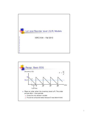
Esma Gel, Pınar Keskinocak, 2013Lot size/Reorder level (Q,R) ModelsISYE 3104 – Fall 2013Recap: Basic EOQInventory I(t)T QdQR d -d T2T3T4TtimeLead time Place an order when the inventory level is R. The orderarrives after time periods Q was the only decision variableR could be computed easily because D was deterministic1
Uncertain demandBoth Q and R are decision variablesCycle time is no longer constant! InventoryQQQRs2s1 s3T1 T2timeT3(Q,R) Decisions We choose R to meet the demand during lead time Service levels: Protect against uncertainties indemand (or lead time)Balance the costs: stock-outs and inventoryTradeoff in Q: Fixed cost versus holding costObjective: Minimize fixed cost holding cost stockout (backorder) cost2
Demand during lead timeInventoryReorderlevelWhat will happen if demandfollows one of these patterns?RExcess inventoryStockoutTime Demand during lead timeInventoryOften the probability distributionof demand during lead timefollows a Normal patternRP(D R) Probabilityof stockout TimeExpected demandduring lead timeR3
(Q,R) Model Assumptions Continuous reviewDemand is random and stationary. Expected demand is d perunit time.Lead time is Costs K: Setup cost per orderh: Holding cost per unit per unit timec: Purchase price (cost) per unitp: Stockout (backorder) cost per unitDemand during lead time is a continuous random variable Dwith pdf (density function) f(x) and cdf (distribution function) F(x)Mean and standard deviation (Q,R) Model – Expected total cost per unit timeHolding costcost Fixed cost ShortageKn( R )Q Q C (Q) h s pRecap : T 2 TTd s Average inventory level before an order arrives (Reorder level) (expected demand during leadtime) R- n( R ) Expected shortage per cycleD R shortage D-RD R shortage 0R 0RRStandard lossfunctionn( R ) 0 f ( x)dx ( x R ) f ( x)dx ( x R ) f ( x)dx L( z )4
(Q,R) Model – Expected total cost per unit timeHolding costcost Fixed cost ShortageKn( R )Q Q C (Q) h s pRecap : T 2 TTd s Average inventory level before an order arrives (Reorder level) (expected demand during leadtime) R- n( R ) Expected shortage per cycleD R shortage D-RD R shortage 0R 0RRStandard lossfunctionn( R ) 0 f ( x)dx ( x R ) f ( x)dx ( x R ) f ( x)dx L( z )(Q,R) Model – Expected total cost per unit timeHolding costcost Fixed cost ShortageKn( R )Q Q C (Q) h s pRecap : T 2 TTd Same expression ass Average inventory level before an order arrivesthe “expected (Reorder level) (expecteddemandnumberofduring leadtime) R- n( R ) Expected shortage per cyclestockouts” in thenewsvendor model(Q replaced by R)D R shortage D-RD R shortage 0R 0RRStandard lossfunctionn( R ) 0 f ( x)dx ( x R ) f ( x)dx ( x R ) f ( x)dx L( z )5
(Q,R) Model – Expected total cost per unit timeG (Q) Holding cost Fixed cost Shortage costdd n( R ) Q h R d K pQQ 2 h d [ K pn( R)] G h Kd pdn( R ) 2 0 22 Q 2 QQQ22d [ K pn( R)]hpd (1 F ( R))Qh G h 1 F ( R) Qpd RQ (Q,R) Model – Expected total cost per unit timeC (Q) Holdingcost Fixed cost Shortagecostd n( R)d Q h R d K pQQ 2 Optimalsolution:1Q 2d[ K p n( R)]hF ( R) 1 Qhpd2How do we pull Q and R from these equations? Solve iteratively!!6
Solving for optimal Q and R Start with a Q0 value and iterate until the Q valuesconvergeQ0 EOQ2Q1R112Q2Q31R2Remember: To find Q,you need n(R) L(z)Lookup for z in the NormaltablesR3R4Example – Rainbow Colors Rainbow Colors paint store uses a (Q,R) inventory system tocontrol its stock levels. For a popular eggshell latex paint,historical data show that the distribution of monthly demandis approximately Normal, with mean 28 and standarddeviation 8. Replenishment lead time for this paint is about14 weeks. Each can of paint costs the store 6. Althoughexcess demands are backordered, each unit of stockoutcosts about 10 due to bookkeeping and loss-of-goodwill.Fixed cost of replenishment is 15 per order and holdingcosts are based on a 30% annual interest rate. What is the optimal lot size (order quantity) and reorder level?What is the expected inventory level (safety stock) just beforean order arrives?7
Example – Rainbow Colors Input Monthly demand Normal mean 28 std.dev. 8 14 weeksc 6, p 10, K 15h ic (0.3)(6) 1.8/unit/yearComputed input d ? (Expected annual demand)Expected demand during lead time ? Variance of demand during lead time 2 ?Example – Rainbow Colors Input Monthly demand Normal mean 28 std.dev. 8 14 weeksc 6, p 10, K 15h ic (0.3)(6) 1.8/unit/yearComputed input d (28)(12) 336 units/year (Expected annual demand)Expected demand during lead time 336 units/year (14 weeks) 90 units52 weeks/yearVariance of demand during lead timeAnnual variance (12)(82 ) 768Variance of lead time demand 768 14 206.77 14.38528
Example – Rainbow Colors Input Monthly demand Normal mean 28 std.dev. 8 14 weeksc 6, p 10, K 15h ic (0.3)(6) 1.8/unit/yearComputed input d (28)(12) 336 units/year (Expected annual demand)Expected demand during lead time (28)(12) units/year (14 weeks) 90 units52 weeks/yearVariance of demand during lead timeAnnual variance (12)(82 ) 768Variance of lead time demand 768 14 206.77 14.3852Example – Rainbow Colors InputMonthly demand Normal mean 28 std.dev. 8 14 weeks c 6,p 10, K 15As the lead time increases, so does the mean and variance h ic (0.3)(6) 1.8/unit/year of demand during lead time Computed inputd (28)(12) 336 units/year (Expected annual demand)Shorter leadtimes Less variability of demand during lead timeExpected demand during lead time (28)(12) units/year (14 weeks) 90 units52 weeks/yearVariance of demand during lead timeAnnual variance (12)(82 ) 768Variance of lead time demand 768 14 206.77 14.38529
Example – Rainbow Colors Iteration 0: Compute EOQQ0 2Kd(2)(15)(336) 75h1.8Example – Rainbow Colors Iteration 1: Compute R1 (given Q0) and then compute Q1(given R1)2F ( R1 ) 1 Q0 h(75)(1.8) 1 0.96 ( z) z 1.75pd(10)(336)From standardNormal table D R Recap: F ( R) P( D R) P P(Z z) ( z ) z R SafetyStockZzStandard Normal R z R1 (14.38)(1.75) 90 115ExpectedDemand duringLead timeQ0 752Q11R1 11510
Example – Rainbow Colors Iteration 1 (continued): Compute Q1 (given R1)2d[ K p n( R)] 1hn( R1 ) L( z) (14.38)(0.0162) 0.233Q Q1 (2)(336)[15 (10)(0.233)] 801.8Q0 75Q1 8021R1 1152R2Q0 and Q1 not close, continue iterationsExample – Rainbow Colors Iteration 2: Compute R2 (given Q1) and then compute Q2(given R2)Q1h(80)(1.8) 1 0.957 ( z ) z 1.72pd(10)(336)R z R2 (14.38)(1.72) 90 115F ( R2 ) 1 Q0 75Q1 80R1 115R2 115STOP! R values converged, optimal (Q,R) (80,115)11
Example – Rainbow Colors (Q,R) (80,115) Reorder level is larger than expected demand duringlead time. Why?Optimal order quantity is larger than EOQ. Why?Safety stock s R- 115-90 25 unitsWeekly demand 5.64Avg cycle time T Q/d 80/6.64 12.38 weeks.Lead time 14 weeks. Cycle time shorter than lead timeImpact of R on the costs and QR inventory , therefore Q QTotal costAs R Q Holding costFixed costShortage costR11511512
Optimal R as a function of QF ( R) 1 QhpdAs the order quantity increases, the reorder leveldecreasesQ holding cost and setup cost , therefore R sothat we can bring the holding cost , although a lower Rmeans shortage cost The Impact of Holding Cost on the Optimal(Q,R)As h goes up, both Q and R go down, but in this exampleQ drops at a faster 75511113
The Impact of Stockout Cost on the Optimal(Q,R)As p goes up, Q goes ? and R goes ?The Impact of Stockout Cost on the Optimal(Q,R)As p goes up, Q goes down and R goes up!pQR284101681111108111514811171880118228012014
Summary: (Q,R) Models Balance between holding cost, setup/fixed cost,and shortage cost To save on the shortage cost, we want large RTo save on the holding cost, we want small Q andsmall RTo save on the fixed cost, we want large QChoose Q and R to strike a good balance amongthese three costs!!! Esma Gel, Pınar Keskinocak, 2013Service Levels in (Q,R) ModelsISYE 3104 – Fall 201315
Service objectives Type I service level ( ) The proportion of cycles in which no stockouts occurExample: 90% Type I service level There are nostockouts in 9 out of 10 cycles (on average)Type II service level (fill rate, ) Fraction of demand satisfied on timeService objectives - ExampleOrder 160401450Stock-outs00450010000055Fraction of periodswith no stock-outs 8/10 Type I service 80% 0.8Fraction of demandsatisfied on time (1450-55)/1450 0.96 Type II service 96% 0.96In general, is it easier to achieve an x% Type I service or Type II service level?16
Type I service level, : Long-run average proportion of cycles with no stock-outs : Probability of having no stock-outs in a cycle : Probability of having no stock-outs during lead time : Probability that demand during lead time is less than R !!! P( D R) D R Recap : P ( D R ) P P( Z z ) ( z ) Set Q EOQFind z that satisfies (z) Set R z (safety stock expected demand during lead time)Type I service level, : Long-run average proportion of cycles with no stock-outs : Probability of having no stock-outs in a cycle : Probability of having no stock-outs during lead time : Probability that demand during lead time is less than R !!! P( D R) D R Recap : P ( D R ) P P( Z z ) ( z ) Set Q EOQFind z that satisfies (z) Set R z (safety stock expected demand during lead time)17
Type I service level, : Long-run average proportion of cycles with no stock-outs : Probability of having no stock-outs in a cycle : Probability of having no stock-outs during lead time : Probability that demand during lead time is less than R !!! P( D R)Why is Q EOQ optimal in this case? D R Recap : P ( D R ) P P( Z z ) ( z ) Set Q EOQFind z that satisfies (z) Set R z (safety stock expected demand during lead time)Example – Rainbow Colors Rainbow Colors paint store uses a (Q,R) inventory system tocontrol its stock levels. For a popular eggshell latex paint,historical data show that the distribution of monthly demandis approximately Normal, with mean 28 and standarddeviation 8. Replenishment lead time for this paint is about14 weeks. Each can of paint costs the store 6. Althoughexcess demands are backordered, each unit of stockoutcosts about 10 due to bookkeeping and loss-of-goodwill.Fixed cost of replenishment is 15 per order and holdingcosts are based on a 30% annual interest rate. What is the optimal lot size (order quantity) and reorder level?What is the expected inventory level (safety stock) just beforean order arrives?18
Example – Rainbow Colors Rainbow Colors is not sure whether the 10estimate for the shortage cost is accurate. Hence,they decided to use a service level approach.What are the optimal (Q,R) values if they want to achieve no stockouts in 90% of the order cycles?satisfy 90% of the demand on time?Example – Rainbow Colors Input Monthly demand Normal mean 28 std.dev. 8 14 weeks, c 6, K 15h Ic (0.3)(6) 1.8/unit/year 0.9 or 0.9Computed input d (28)(12) 336 units/year (Expected annual demand)Expected demand during lead time (28)(12) units / year (14 weeks) 90 units52 weeks / yearVariance of demand during lead time Annual variance (12)(82 ) 768Variance of lead time demand 768 14 206.77 14.385219
Rainbow Colors – Type I serviceFind (Q,R) to have 90% Type I service level Q EOQ 75 (z) 0.9 z 1.28R z R (14.38)(1.28) 90 108For 90% Type I service level (Q,R) (75,108)Remember: With unit penalty cost of 10, we found (Q,R) (80,115).What is the Type I service level that corresponds to(Q,R) (80,115)?R z 115 (14.38)z 90 z 1.7385 (1.7385) 0.96 96% Type I service level when (Q,R) (80,115)Type II service level : Fraction of demand met on time1- : Fraction of demand not met on time (stock-outs)Recap:Expected # of stockouts per unit time 1 n( R ) d n ( R ) TQQ since T d Expected # of stockouts per unit time n( R)n( R )4 1 Expected demand per unit timeQQWith this information, for a given (Q,R), we can compute .20
Rainbow Colors For 90% Type I service level we found(Q,R) (75,108)What is the Type II service level which correspondsto this policy?The same policy results in 90% Type Iservice and 99% Type II service!!R 108 90 1.25 z14.38 n( R ) L( z ) L (1.25) (14.38)(0.0506) 0.7276n( R ) 0.72761 0.0097 0.9975Q Finding the optimal (Q,R) for a desired Type IIservice levelRemember : Optimal solution when we havestock - out cost p :1Q 2d [ K p n( R)]hF ( R) 1 Qhpd221
Finding the optimal (Q,R) for a desired Type IIservice levelOptimal solution when we have stock - out cost p :1Q 2d [ K p n( R )]hp From 2 :F ( R) 1 Qhd 1 F ( R) Qhpd25 Imputed shortage costSubstitute p into 1 :2n( R )2 Kd n( R ) 3 Q hFR1 F ( R)1() To be solved simultaneously with n( R) (1 )Q4Impact of service level on R For a given Q As n(R) (1- )Q i.e., R As the service level , the reorder level as well22
Finding the optimal (Q,R) for a desired Type IIservice leveln( R )2 Kd n( R) Q 1 F ( R)h 1 F ( R) 23n( R ) (1 )Q4Q0 EOQ4Q13R14Q23R2 Start with a Q0 value anditerate until the Q values(or the R values) converge4Q3R334R4Example – Rainbow Colors Iteration 0: Compute EOQQ0 2Kd(2)(15)(336) 75h1.823
Example – Rainbow Colors Iteration 1: Compute R1 (given Q0) and then compute Q1(given R1)n( R1 ) (1 )Q0 (1 0.9)(75) 7.5 L( z) 4L( z) 0.5216 z 0.22R1 z (14.38)( 0.22) 90 86.83 87To find Q1 we need 1-F ( R1 ). Look at the Normal table.1 F ( 0.22) F (0.22) 0.5871Q1 893Q0 754Q1 893R1 87Example – Rainbow Colors Iteration 2: Compute R2 (given Q1) and then compute Q2(given R2)24
Example – Rainbow Colors Iteration 2: Compute R2 (given Q1) and then compute Q2(given R2)n( R2 ) (1 )Q1 (1 0.9)(89) 8.9 L( z) 4L( z) 0.619 z 0.38R2 z (14.38)( 0.38) 90 84.5 85To find Q1 we need 1-F ( R1 ). Look at the Normal table.1 F ( 0.38) F (0.38) 0.648Q0 754Q2 90Q1 893R1 8734Q2 90R2 853Example – Rainbow Colors Iteration 3: Compute R3 (given Q2) and then compute Q3(given R3)n( R3 ) (1 )Q2 (1 0.9)(85) 8.5 L( z) L( z) 0.591 z 0.34R3 z (14.38)( 0.34) 90 85.1 854Q0 754Q1 89R1 8734Q2 90STOP! R values converged, optimal (Q,R) (90,85)R2 8534R3 8525
2 Uncertain demand Both Q and R are decision variables Cycle time is no longer constant! Inventory R Q Q s1 s2 Q s3 T1 T2 T3 time (Q,R) Decisions We choose R to meet the demand during lead time Service levels: Protect against uncertainties in demand (or lead time) Balance the costs: stock-outs and inventory Tradeoff in Q: Fixed cost versus holding cost