Transcription
Essentials of Modern Business Statistics with Microsoft Office Excel 7th Edition Anderson Solutions ManualFull Download: xcel-7th-editChapter 3Descriptive Statistics: Numerical MeasuresLearning Objectives1.Understand the purpose of measures of location.2.Be able to compute the mean, weighted mean, geometric mean, median, mode, quartiles, and variouspercentiles.3.Understand the purpose of measures of variability.4.Be able to compute the range, interquartile range, variance, standard deviation, and coefficient ofvariation.5.Understand skewness as a measure of the shape of a data distribution. Learn how to recognize when adata distribution is negatively skewed, roughly symmetric, and positively skewed.6.Understand how z scores are computed and how they are used as a measure of relative location of adata value.7.Know how Chebyshev’s theorem and the empirical rule can be used to determine the percentage ofthe data within a specified number of standard deviations from the mean.8.Learn how to construct a 5–number summary and a box plot.9.Be able to compute and interpret covariance and correlation as measures of association between twovariables.10.Understand the role of summary measures in data dashboards.3-1 2015 Cengage Learning. All Rights Reserved.May not be scanned, copied or duplicated, or posted to a publicly accessible website, in whole or in part.This sample only, Download all chapters at: AlibabaDownload.com
Chapter 3Solutions:x 1. xi 75 15n510, 12, 16, 17, 20Median 16 (middle value)x 2. xi 96 16n610, 12, 16, 17, 20, 21Median 3.16 17 16.52 wi xi 6(3.2) 3(2) 2(2.5) 8(5) 70.2 3.69 wi6 3 2 819a.x b.3.2 2 2.5 5 12.7 3175.444.Period12345Rate of Return (%)-6.0-8.0-4.02.05.4The mean growth factor over the five periods is:xg n x1 x2 x5 5 0.940 0.920 0.960 1.020 1.054 5 0.8925 0.9775So the mean growth rate (0.9775 – 1)100% –2.25%.5.15, 20, 25, 25, 27, 28, 30, 34L20 p20(n 1) (8 1) 1.810010020th percentile 15 .8(20 ̶ 15) 19L25 p25(n 1) (8 1) 2.2510010025th percentile 20 .25(25 ̶ 20) 21.25L65 p65(n 1) (8 1) 5.851001003-2 2015 Cengage Learning. All Rights Reserved.May not be scanned, copied or duplicated, or posted to a publicly accessible website, in whole or in part.
Descriptive Statistics: Numerical Measures65th percentile 27 .85(28 ̶ 27) 27.85L75 p75(n 1) (8 1) 6.7510010075th percentile 28 .75(30 ̶ 28) 29.5Mean 6.7. xi 657 59.73n11Median 576th itemMode 53It appears 3 timesa.The mean commute time is 1291.5/48 26.91 minutes.b.The median commute time is 25.95 minutes.c.The data are bimodal. The modes are 23.4 and 24.8.d.L75 p75(n 1) (48 1) 36.7510010075th percentile 28.5 .75(28.5 ̶ 28.5) 28.58.a.Median 80 or 80,000. The median salary for the sample of 15 middle-level managers working atfirms in Atlanta is slightly lower than the median salary reported by the Wall Street Journal.b.x xi 1260 84n15Mean salary is 84,000. The sample mean salary for the sample of 15 middle-level managers isgreater than the median salary. This indicates that the distribution of salaries for middle-levelmanagers working at firms in Atlanta is positively skewed.c.The sorted data are as follows:53L25 55636773757780838593106108118124p25(n 1) (16) 4100100First quartile or 25th percentile is the value in position 4 or 67.L75 p75(n 1) (16) 12100100Third quartile or 75th percentile is the value in position 12 or 106.9. xi 30.57 2.55n12a.x b.Order the data from low 1.88 to high 5.003-3 2015 Cengage Learning. All Rights Reserved.May not be scanned, copied or duplicated, or posted to a publicly accessible website, in whole or in part.
Chapter 3Use 6th and 7th positions.Median c.2.34 2.19 2.2652 25 L.25 (12 1) 3.25 Q1 1.97 .25(2.09-1.97) 2.0 100 75 L.75 (12 1) 9.75 Q3 2.56 .75(2.91-2.56) 2.8225 100 10. a.x xin 1318 65.920Order the data from the lowest rating (42) to the highest rating (83)PositionL50 11571661167176217768631878964198110662083p50( n 1) (20 1) 10.5100100Median or 50th percentile 66 . 5(67 ̶ 66) 66.5Mode is 61.b.L25 p25(n 1) (20 1) 5.25100100First quartile or 25th percentile 61L75 p75(n 1) (20 1) 15.75100100Third quartile or 75th percentile 71c.L90 p90(n 1) (20 1) 18.910010090th percentile 78 .9(81 ̶ 78) 80.73-4 2015 Cengage Learning. All Rights Reserved.May not be scanned, copied or duplicated, or posted to a publicly accessible website, in whole or in part.
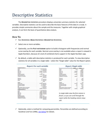
Descriptive Statistics: Numerical Measures90% of the ratings are 80.7 or less;10% of the ratings are 80.7 or greater.11. a.The median number of hours worked per week for high school science teachers is 54.b.The median number of hours worked per week for high school English teachers is 47.c.The median number of hours worked per week for high school science teachers is greater than themedian number of hours worked per week for high school English teachers; the difference is 54 – 47 7 hours.12. a.The minimum number of viewers that watched a new episode is 13.3 million, and the maximumnumber is 16.5 million.b.The mean number of viewers that watched a new episode is 15.04 million or approximately 15.0million; the median also 15.0 million. The data is multimodal (13.6, 14.0, 16.1, and 16.2 million); insuch cases the mode is usually not reported.c.The data are first arranged in ascending order.L25 p25(n 1) (21 1) 5.50100100First quartile or 25th percentile 14 .50(14.1 ̶ 14) 14.05L75 p75(n 1) (21 1) 16.5100100Third quartile or 75th percentile 16 . 5(16.1 ̶ 16) 16.05A graph showing the viewership data over the air dates follows. Period 1 corresponds to the firstepisode of the season, period 2 corresponds to the second episode, and so on.18.016.014.0Viewers dThis graph shows that viewership of The Big Bang Theory has been relatively stable over the 2011–2012 television season.3-5 2015 Cengage Learning. All Rights Reserved.May not be scanned, copied or duplicated, or posted to a publicly accessible website, in whole or in part.
Chapter 313.Using the mean we get xcity 15.58, xhighway 18.92For the samples we see that the mean mileage is better on the highway than in the city.City13.2 14.4 15.2 15.3 15.3 15.3 15.9 16 16.1 16.2 16.2 16.7 16.8 MedianMode: 15.3Highway17.2 17.4 18.3 18.5 18.6 18.6 18.7 19.0 19.2 19.4 19.4 20.6 21.1 MedianMode: 18.6, 19.4The median and modal mileages are also better on the highway than in the city.14.For March 2011:L25 p25(n 1) (50 1) 12.75100100First quartile or 25th percentile 6.8 .75(6.8 ̶ 6.8) 6.8L50 p50(n 1) (50 1) 25.5100100Second quartile or median 8 .5(8 ̶ 8) 8L75 p75(n 1) (50 1) 38.25100100Third quartile or 75th percentile 9.4 . 25(9.6 ̶ 9.4) 9.45For March 2012:L25 p25(n 1) (50 1) 12.75100100First quartile or 25th percentile 6.2 .75(6.2 ̶ 6.2) 6.2L50 p50(n 1) (50 1) 25.5100100Second quartile or median 7.3 .5(7.4 ̶ 7.3) 7.35L75 p75(n 1) (50 1) 38.25100100Third quartile or 75th percentile 8.6 . 25(8.6 ̶ 8.6) 8.63-6 2015 Cengage Learning. All Rights Reserved.May not be scanned, copied or duplicated, or posted to a publicly accessible website, in whole or in part.
Descriptive Statistics: Numerical MeasuresIt may be easier to compare these results if we place them in a table.March 20116.808.009.45First QuartileMedianThird QuartileMarch 20126.207.358.60The results show that in March 2012 approximately 25% of the states had an unemployment rate of6.2% or less, lower than in March 2011. And, the median of 7.35% and the third quartile of 8.6% inMarch 2012 are both less than the corresponding values in March 2011, indicating thatunemployment rates across the states are decreasing.15.To calculate the average sales price we must compute a weighted mean. The weighted mean is501 34.99 1425 38.99 294 36.00 882 33.59 715 40.99 1088 38.59 1644 39.59 819 37.99 501 1425 294 882 715 1088 1644 819 38.11Thus, the average sales price per case is 38.11.16. a.Grade xi4 (A)3 (B)2 (C)1 (D)0 (F)x w x wi i ib.17. a.Weight wi915333060 Credit Hours9(4) 15(3) 33(2) 3(1) 150 2.509 15 33 360Yes; satisfies the 2.5 grade point average requirementx w x wi i 9191(4.65) 2621(18.15) 1419(11.36) 2900(6.75)9191 2621 1419 2900 126, 004.14 7.8116,131iThe weighted average total return for the Morningstar funds is 7.81%.b.If the amount invested in each fund was available, it would be better to use those amounts asweights. The weighted return computed in part (a) will be a good approximation, if the amountinvested in the various funds is approximately equal.c.Portfolio Return 2000(4.65) 4000(18.15) 3000(11.36) 1000(6.75)2000 4000 3000 1000122, 730 12.2710, 0003-7 2015 Cengage Learning. All Rights Reserved.May not be scanned, copied or duplicated, or posted to a publicly accessible website, in whole or in part.
Chapter 3The portfolio return would be 12.27%.18.Assessment54321Totalx Deans:Deans446660100180 w x w 684 3.8180 w x w 444 3.7120i iix Recruiters:i 136129240444Business school deans rated the overall academic quality of master’s programs slightly higher than corporaterecruiters did.19.To calculate the mean growth rate we must first compute the geometric mean of the five growthfactors:xg Year2007% Growth5.5Growth Factor 18n1.055 x1 x2 x5 5 1.055 1.011 0.965 0.989 1.018 5 1.036275 1.007152The mean annual growth rate is (1.007152 – 1)100 0.7152%.20.YearYear1StiversEnd of YearGrowthValueFactor 11,0001.100TrippiEnd of YearGrowthValueFactor 5,6001.120Year 2 12,0001.091 6,3001.125Year 3 13,0001.083 6,9001.095Year 4 14,0001.077 7,6001.101Year 5 15,0001.071 8,5001.118Year 6 16,0001.067 9,2001.082Year 7 17,0001.063 9,9001.076Year 8 18,0001.059 10,6001.0713-8 2015 Cengage Learning. All Rights Reserved.May not be scanned, copied or duplicated, or posted to a publicly accessible website, in whole or in part.
Descriptive Statistics: Numerical MeasuresFor the Stivers mutual fund we have:18000 10000 x1 x2 xg n x8 , so x1 x2 x8 1.8 and x1 x2 x8 8 1.80 1.07624So the mean annual return for the Stivers mutual fund is (1.07624 – 1)100 7.624%For the Trippi mutual fund we have:10600 5000 x1 x2 xg n x8 , so x1 x2 x8 2.12 and x1 x2 x8 8 2.12 1.09848So the mean annual return for the Trippi mutual fund is (1.09848 – 1)100 9.848%.While the Stivers mutual fund has generated a nice annual return of 7.6%, the annual return of 9.8%earned by the Trippi mutual fund is far superior.21.3500 5000 x1 x2 xg n x9 , so x1 x2 x9 0.7, and so x1 x2 x9 9 .7 .961144So the mean annual growth rate is ( 0.961144 – 1)100 -3.8856%22.25,000,000 10,000,000 x1 x2 xg n x6 , so x1 x2 x6 2.50, and so x1 x2 x6 6 2.50 1.165So the mean annual growth rate is (1.165 – 1)100 16.5%23.Range 20 - 10 1010, 12, 16, 17, 20L25 p25(n 1) (6) 1.5100100First Quartile or Q1 10 .5(12-10) 11L75 p75(n 1) (6) 4.5100100Third Quartile or Q3 17 .5(20-17) 18.5IQR Q3 – Q1 18.5 – 11 7.524.x xi 75 15n53-9 2015 Cengage Learning. All Rights Reserved.May not be scanned, copied or duplicated, or posted to a publicly accessible website, in whole or in part.
Chapter 3 ( xi x ) 2 64 16n 14s2 s 16 425.15, 20, 25, 25, 27, 28, 30, 34L25 Range 34 – 15 19p25(n 1) (9) 2.25100100First Quartile or Q1 20 .25(25-20) 21.25L75 p75(n 1) (9) 6.75100100Third Quartile or Q3 28 .75(30-28) 29.5IQR Q3 – Q1 29.5 – 21.25 8.25 xi 204 255.n8x s2 ( xi x ) 2 242 34.57n 17s 34.57 5.88 x74.4 3.722026. a.x b.s c.The average price for a gallon of unleaded gasoline in San Francisco is much higher than thenational average. This indicates that the cost of living in San Francisco is higher than it would be forcities that have an average price close to the national average.iin ( x x )iin 12 1.6516 .0869 .294820 127. a.The mean price for a round–trip flight into Atlanta is 356.73, and the mean price for a round–tripflight into Salt Lake City is 400.95. Flights into Atlanta are less expensive than flights into SaltLake City. This possibly could be explained by the locations of these two cities relative to the 14departure cities; Atlanta is generally closer than Salt Lake City to the departure cities.b.For flights into Atlanta, the range is 290.0, the variance is 5517.41, and the standard Deviation is 74.28. For flights into Salt Lake City, the range is 458.8, the variance is 18933.32, and thestandard deviation is 137.60.The prices for round–trip flights into Atlanta are less variable than prices for round–trip flights intoSalt Lake City. This could also be explained by Atlanta’s relative nearness to the 14 departure cities.3 - 10 2015 Cengage Learning. All Rights Reserved.May not be scanned, copied or duplicated, or posted to a publicly accessible website, in whole or in part.
Descriptive Statistics: Numerical Measures28. a.The mean serve speed is 180.95, the variance is 21.42, and the standard deviation is 4.63.b.29. a.Although the mean serve speed for the twenty Women's Singles serve speed leaders for the 2011Wimbledon tournament is slightly higher, the difference is very small. Furthermore, given thevariation in the twenty Women's Singles serve speed leaders from the 2012 Australian Open and thetwenty Women's Singles serve speed leaders from the 2011 Wimbledon tournament, the differencein the mean serve speeds is most likely due to random variation in the players’ performances.Range 60 – 28 3228 42 45 48 49 50 55 58 60L25 p25(n 1) (10) 2.5100100First Quartile or Q1 42 .5(45-42) 43.5p75(n 1) (10) 7.5100100Third Quartile or Q3 55 .5(58-55) 56.5L75 IQR Q3 – Q1 b.x 56.5 - 43.5 13435 48.339 ( xi x ) 2 742s2 ( xi x ) 2 742 92.75n 18s 92.75 9.63c.30.The average air quality is about the same. But, the variability is greater in Anaheim.Dawson Supply: Range 11 – 9 24.1 0.679J.C. Clark: Range 15 – 7 8s s 60.1 2.58931. a.meanmedianstandard 82.5431.745 1070.41163.5334.5The 45 group appears to spend less on coffee than the other two groups, and the 18–34 and 35–44groups spend similar amounts of coffee.3 - 11 2015 Cengage Learning. All Rights Reserved.May not be scanned, copied or duplicated, or posted to a publicly accessible website, in whole or in part.
Chapter 332. a.b.Automotive:x xDepartment store:x xAutomotive:s (x x )Department store:s (x x )inin 39201 1960.0520 13857 692.85202i(n 1)i(n 1) 4, 407, 720.95 481.6519 456804.55 155.06192c.Automotive:2901 – 598 2303Department Store: 1011 – 448 563d.Order the data for each variable from the lowest to highest.1234567891011121314151617181920L25 014202420582166220222542366252625312901Department 8248408569471011p25(n 1) (21) 5.25100100Automotive: First quartile or 25th percentile 1714 .25(1720 – 1714) 1715.5Department Store: First quartile or 25th percentile 589 .25(597 – 589) 5913 - 12 2015 Cengage Learning. All Rights Reserved.May not be scanned, copied or duplicated, or posted to a publicly accessible website, in whole or in part.
Descriptive Statistics: Numerical MeasuresL75 p75(n 1) (21) 15.75100100Automotive: Third quartile or 75th percentile 2202 .75(2254 – 2202) 2241Department Store: First quartile or 75th percentile 782 .75(824 – 782) 813.5Automotive IQR Q3 –Q1 2241 - 1715.5 525.5Department Store IQR Q3 –Q1 813.5 - 591 222.5e.33. a.Automotive spends more on average, has a larger standard deviation, larger max and min, and largerrange than Department Store. Autos have all new model years and may spend more heavily onadvertising.For 2014x s xi 608 76n8 ( xi x ) 230 2.07n 17For 2015x s b.34. xi 608 76n8 ( xi x ) 2194 5.26n 17The mean score is 76 for both years, but there is an increase in the standard deviation for the scoresin 2015. The golfer is not as consistent in 2015 and shows a sizeable increase in the variation withgolf scores ranging from 71 to 85. The increase in variation might be explained by the golfer tryingto change or modify the golf swing. In general, a loss of consistency and an increase in the standarddeviation could be viewed as a poorer performance in 2015. The optimism in 2015 is that three ofthe eight scores were better than any score reported for 2014. If the golfer can work for consistency,eliminate the high score rounds, and reduce the standard deviation, golf scores should showimprovement.Quarter milerss 0.0564Coefficient of Variation (s/ x )100% (0.0564/0.966)100% 5.8%Milerss 0.1295Coefficient of Variation (s/ x )100% (0.1295/4.534)100% 2.9%Yes; the coefficient of variation shows that as a percentage of the mean the quarter milers’ timesshow more variability.3 - 13 2015 Cengage Learning. All Rights Reserved.May not be scanned, copied or duplicated, or posted to a publicly accessible website, in whole or in part.
Chapter 3 xi 75 15n5x 35.s2 ( xi x ) 2 n 110z 10 15 1.25420z 20 15 1.25412z 12 15 .75417z 17 15 .50464 4416 15 .254520 500z .201001636.z z 650 500 1.50100z 500 500 0.00100z 450 500 .50100z 280 500 2.2010037. a.z 20 3040 30 2, z 2551 1 .75 At least 75%22b.z 15 3045 30 3, z 3551 1 .89 At least 89%32c.z 22 3038 30 1.6, z 1.6551 1 .61 At least 61%1.62d.z 18 3042 30 2.4, z 2.4551 1 .83 At least 83%2.423 - 14 2015 Cengage Learning. All Rights Reserved.May not be scanned, copied or duplicated, or posted to a publicly accessible website, in whole or in part.
Descriptive Statistics: Numerical Measurese.38. a.z 12 3048 30 3.6, z 3.6551 .92 At least 92%3.62Approximately 95%b.Almost allc.Approximately 68%39. a.1 This is from 2 standard deviations below the mean to 2 standard deviations above the mean.With z 2, Chebyshev’s theorem gives:1 111 3 1 2 1 .752z24 4Therefore, at least 75% of adults sleep between 4.5 and 9.3 hours per day.b.This is from 2.5 standard deviations below the mean to 2.5 standard deviations above the mean.With z 2.5, Chebyshev’s theorem gives:111 1 1 .84226.25z2.5Therefore, at least 84% of adults sleep between 3.9 and 9.9 hours per day.1 c.With z 2, the empirical rule suggests that 95% of adults sleep between 4.5and 9.3 hours per day.The percentage obtained using the empirical rule is greater than the percentage obtained usingChebyshev’s theorem.40. a. 3.33 is one standard deviation below the mean and 3.53 is one standard deviation above the mean.The empirical rule says that approximately 68% of gasoline sales are in this price range.b.Part (a) shows that approximately 68% of the gasoline sales are between 3.33 and 3.53. Since thebell-shaped distribution is symmetric, approximately half of 68%, or 34%, of the gasoline salesshould be between 3.33 and the mean price of 3.43. 3.63 is two standard deviations above themean price of 3.43. The empirical rule says that approximately 95% of the gasoline sales should bewithin two standard deviations of the mean. Thus, approximately half of 95%, or 47.5%, of thegasoline sales should be between the mean price of 3.43 and 3.63. The percentage of gasolinesales between 3.33 and 3.63 should be approximately 34% 47.5% 81.5%. 3.63 is two standard deviations above the mean and the empirical rule says that approximately 95%of the gasoline sales should be within two standard deviations of the mean. Thus, 1 – 95% 5% ofthe gasoline sales should be more than two standard deviations from the mean. Since the bell-shapeddistribution is symmetric, we expected half of 5%, or 2.5%, would be more than 3.63.c.41. a.b.647 is one standard deviation above the mean. Approximately 68% of the scores are between 447and 647 with half of 68%, or 34%, of the scores between the mean of 547 and 647. Also, since thedistribution is symmetric, 50% of the scores are above the mean of 547. With 50% of the scoresabove 547 and with 34% of the scores between 547 and 647, 50% – 34% 16% of the scores are647 or higher.747 is two standard deviations above the mean. Approximately 95% of the scores are between 347and 747 with half of 95%, or 47.5%, of the scores between the mean of 547 and 747. Also, since thedistribution is symmetric, 50% of the scores are above the mean of 547. With 50% of the scores3 - 15 2015 Cengage Learning. All Rights Reserved.May not be scanned, copied or duplicated, or posted to a publicly accessible website, in whole or in part.
Chapter 3above 547 and with 47.5% of the scores between 547 and 747, 50%– 47.5% 2.5% of the scores are747 or higher.c.Approximately 68% of the scores are between 447 and 647 with half of 68%, or 34%, of the scoresare between 447 and the mean of 547.d.Approximately 95% of the scores are between 347 and 747 with half of 95%, or 47.5%, of the scoresbetween 347 and the mean of 547. Approximately 68% of the scores are between 447 and 647 withhalf of 68%, or 34%, of the scores between the mean of 547 and 647. Thus, 47.5% 34% 81.5%of the scores are between 347 and 647.x 2300 3100 .671200 4900 3100 1.50120042. a.z b.z c. 2300 is .67 standard deviations below the mean. 4900 is 1.50 standard deviations above the mean.Neither is an outlier.d.z x x 13000 3100 8.251200 13,000 is 8.25 standard deviations above the mean. This cost is an outlier.43. a.x xi 106.5 10.65n10Median 10.7Mode 10.7b.Range 11.8 – 8.3 3.5s2 ( xi x ) 2 8.085 .8983n 19s .8983 .9478c.For the response time of 8.3, the z-score is z 8.3 10.65 2.4794.9478Thus, this observation does not appear to be an outlier.d.44. a.The national standard of six minutes is not being met for this neighborhood. The city shouldconsider making changes in its response strategy including relocating stations to reduce the traveltime.x xi 765 76.5n103 - 16 2015 Cengage Learning. All Rights Reserved.May not be scanned, copied or duplicated, or posted to a publicly accessible website, in whole or in part.
Descriptive Statistics: Numerical Measures ( xi x ) 2442.5 7 .01n 110 1s b.z x x 84 76.5 1.07s7.01Approximately one standard deviation above the mean. Approximately 68% of the scores are withinone standard deviation. Thus, half of the remaining 32%, or 16%, of the games should have awinning score of more than one standard deviation above the mean or a score of 84 or more points.z x x 90 76.5 1.93s7.01Approximately two standard deviations above the mean. Approximately 95% of the scores arewithin two standard deviations. Thus, half of the remaining 5%, or 2.5%, of the games should havea winning score of more than two standard deviations above the mean or a score of more than 90points.c. xi 122 12.2n10x ( xi x ) 2559.6 7.89n 110 1s Smallest margin 3:z Largest margin 24: z 45. a.x x 3 12.2 1.17s7.89x x 24 12.2 1.50 . No outliers.s7.89The data in ascending order follow:36x 3843444445505556565760626569 xi 780 52n15L50 p50(n 1) (15 1) 8100100Median is the value in position 8 or 55.b.L25 p25(n 1) (15 1) 4100100First quartile or 25th percentile is the value in position 4 or 44.L75 p75(n 1) (15 1) 121001003 - 17 2015 Cengage Learning. All Rights Reserved.May not be scanned, copied or duplicated, or posted to a publicly accessible website, in whole or in part.
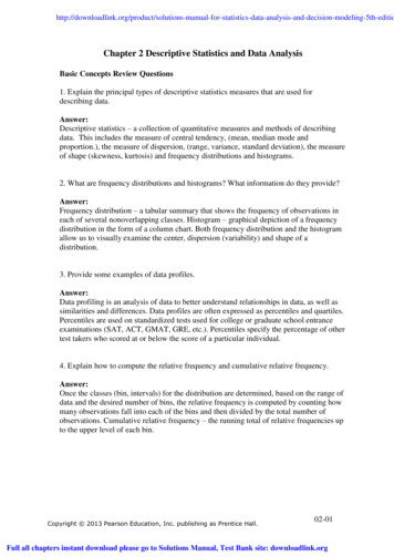
Chapter 3Third quartile or 75th percentile is the value in position 12 or 60.c.The range is 69 – 36 33 and the interquartile range is 60 – 44 16.d.s2 ( xi x ) 2 1402 100.1429n 114s 100.1429 10.007146.e.The z-score values do not indicate any outliers.f.The sample mean of 52% indicates that Wal-Mart does appear to be meeting its goal of reducing thenumber of hourly employees by about 50%.15, 20, 25, 25, 27, 28, 30, 34Smallest 15L25 p25(n 1) (8 1) 2.25100100First quartile or 25th percentile 20 .25(25 ̶ 20) 21.25L50 p50(n 1) (8 1) 4.5100100Second quartile or median 25 .5(27 ̶ 25) 26L75 p75(n 1) (8 1) 6.75100100Third quartile or 75th percentile 28 . 75(30 ̶ 28) 29.5Largest 3447.A box plot created using Excel’s Box and Whisker Statistical Chart follows.3 - 18 2015 Cengage Learning. All Rights Reserved.May not be scanned, copied or duplicated, or posted to a publicly accessible website, in whole or in part.
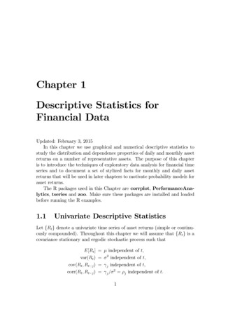
Descriptive Statistics: Numerical Measures48.5, 6, 8, 10, 10, 12, 15, 16, 18Smallest 5L25 p25(n 1) (9 1) 2.5100100First quartile or 25th percentile 6 . 5(8 ̶ 6) 7L50 p50(n 1) (9 1) 5.0100100Second quartile or median 10L75 p75(n 1) (9 1) 7.5100100Third quartile or 75th percentile 15 . 5(16 ̶ 15) 15.5Largest 18A box plot created using Excel’s Box and Whisker Statistical Chart follows.49.IQR 50 – 42 8Lower Limit:Q1 – 1.5 IQR 42 – 12 30Upper Limit:Q3 1.5 IQR 50 12 6265 is an outlier3 - 19 2015 Cengage Learning. All Rights Reserved.May not be scanned, copied or duplicated, or posted to a publicly accessible website, in whole or in part.
Chapter 350. a.b.The first place runner in the men’s group finished 109.03 65.30 43.73 minutes ahead of the firstplace runner in the women’s group. Lauren Wald would have finished in 11 th place for thecombined groups.Using Excel’s MEDIAN function the results are as follows:MenWomen109.64131.67Using the median finish times, the men’s group finished 131.67 109.64 22.03 minutes ahead ofthe women’s group.Also note that the fastest time for a woman runner, 109.03 minutes, is approximately equal to themedian time of 109.64 minutes for the men’s group.c.Using Excel’s QUARTILE.EXC function the quartiles are as .6703129.025147.180Excel’s MIN and MAX functions provided the following 28Five number summary for men: 65.30, 83.1025, 109.640, 129.025, 148.70Five number summary for women: 109.03, 122.08, 131.67, 147.18, 189.28d.Men: IQR 129.025 – 83.1025 45.9225Lower Limit Q1 1.5(IQR) 83.1025 – 1.5(45.9225) 14.22Upper Limit Q3 1.5(IQR) 129.025 1.5(45.9225) 197.91There are no outliers in the men’s group.Women: IQR 147.18 122.08 25.10Lower Limit Q1 1.5(IQR) 122.08 1.5(25.10) 84.43Upper Limit Q3 1.5(IQR) 147.18 1.5(25.10) 184.83The two slowest women runners with times of 189.27 and 189.28 minutes are outliers in thewomen’s group.e.A box plot created using Excel’s Box and Whisker Statistical Chart follows.3 - 20 2015 Cengage Learning. All Rights Reserved.May not be scanned, copied or duplicated, or posted to a publicly accessible website, in whole or in part.
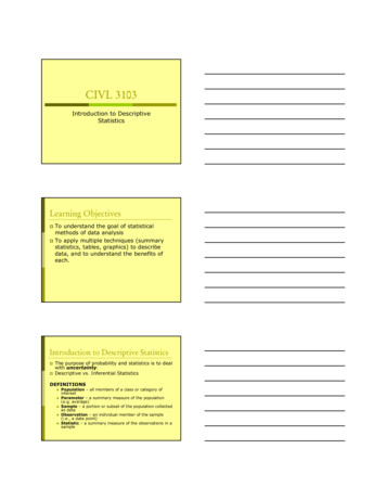
Descriptive Statistics: Numerical MeasuresThe box plots show the men runners with the faster or lower finish times. However, the box plotsshow the women runners with the lower variation in finish times. The interquartile ranges of45.9225 minutes for men and 25.10 minutes for women support this conclusion.51. a.Smallest 608L25 p25(n 1) (21 1) 5.5100100First quartile or 25th percentile 1850 . 5(1872 ̶ 1850) 1861L50 p50(n 1) (21 1) 11.0100100Second quartile or median 4019L75 p75(n 1) (21 1) 16.5100100Third quartile or 75th percentile 8305 . 5(8408 ̶ 8305) 8356.5Largest 14138Five-number summary: 608, 1861, 4019, 8365.5, 14138b.Limits:IQR Q3 – Q1 8356.5 – 1861 6495.5Lower Limit:Q1 – 1.5(IQR) 1861 – 1.5(6495.5) ̶ 7,882.253 - 21 2015 Cengage Learning. All Rights Reserved.May not be scanned, copied or duplicated, or posted to a publicly accessible website, in whole or in part.
Chapter 3Upper Limit:Q3 1.5(IQR) 8356.5 1.5(6495.5) 18,099.75c.There are no outliers, all data are within the limits.d.Yes, if the first two digits in Johnson and Johnson's sales were transposed to 41,138, sales wouldhave shown up as an outlier. A review of the data would have enabled the correction of the data.e.A box plot created using Excel’s Box and Whisker Statistical Chart follows.52.Excel’s MIN, QUARTILE.EXC, and MAX functions provided the following mum66636875First Quartile686571.2577Median716673.578.5Third Quartile7367.7574.7579.75Maximum75697781a.Median for T-Mobile is 73.5b.5- number summary: 68, 71.25, 73.5, 74.75, 77c.IQR Q3 – Q1 74.75 – 71.25 3.5Lower Limit Q1 – 1.5(IQR) 71.25 – 1.5(3.5) 66Upper Limit Q3 1.5(IQR)3 - 22 2015 Cengage Learning. All Rights Reserved.May not be scanned, copied or duplicated, or posted to a publicly accessible website, in whole or in part.
Descriptive Statistics: Numerical Measures 74.75 1.5(3.5) 80All ratings are between 66 and 80. There are no outliers for the T-Mobile service.d.Using the five number summaries shown initially, the limits for the four cell-phone services are rst Quartile686571.2577Median716673.578.5Third 757.54.1255.254.125Lower Limit60.560.8756672.875Upper Limit80.571.8758083.875IQR1.5(IQR)75There are no outliers for any of the cell-phone services.e.A box plot created using Excel’s Box and W
Descriptive Statistics: Numerical Measures Learning Objectives 1. Understand the purpose of measures of location. 2. Be able to compute the mean, weighted mean, geometric mean, median, mode, quartiles, and various . Essentials of Modern Business Statistics with Microsoft Office Excel 7th Edition Anderson Solutions Manual Full Download: https .