Transcription
Open AccessEstimating extreme dry spell risk in Ichkeul Lake Basin(Northern Tunisia): a comparative analysis of annualmaxima series with a Gumbel distributionMajid Mathlouthi1 and Fethi Lebdi21 ResearchLaboratory in Sciences and Technology of Water at National Agronomic Institute of Tunisia,Tunis, 1082, Tunisia2 National Agronomic Institute of Tunisia,Tunis, 1082, TunisiaCorrespondence: Majid Mathlouthi (majid mathlouthi@yahoo.fr)Published: 16 September 2020Abstract. This paper analyses a 42 year time series of daily precipitation in Ichkeul Lake Basin (northernTunisia) in order to predict extreme dry-spell risk. Dry events are considered as a sequence of dry days separatedby rainfall events from each other. Thus the rainy season is defined as a series of rainfall and subsequent dryevents. Rainfall events are defined as the uninterrupted sequence of rainy days, when at last on one day more thana threshold amount of rainfall has been observed. A comparison of observed and estimated maximum dry events(42 year return period) showed that Gumbel distribution fitted to annual maximum series gives better resultsthan the exponential (E) distribution combined with partial duration series (PDS). Indeed, the classical Gumbelapproach slightly underestimated the empirical duration of dry events. The AMS–G approach was successfullyapplied in the study of extreme hydro-climatic variable values. The results reported here could be applied inestimating climatic drought risks in other geographical areas.1IntroductionA proper simulation of precipitation is important. Precipitation is a very important element of climate that affects boththe natural environment and human society. Events rangingfrom prolonged droughts to short-term, high intensity floodsare often associated with devastating impacts both to societyand the environment (Hui et al., 2005). An alternative to theMarkov chain process which is typically used to simulate theoccurrence of precipitation is to use a wet-dry spell modelor alternating renewal model, that is, to simulate wet and dryspells separately by fitting their durations to an appropriateprobability distribution. Among the study using the wet-dryspell approach one can cite, for example, Bogardi and Duckstein (1993); Wilks (1999); Mathlouthi (2009); Mathlouthiand Lebdi (2008, 2009, 2017); Dunxian et al. (2015); Konjitet al., 2016.It is well known that dry spells cause major economic andhuman losses, and numerous studies have highlighted theneed for drought prevention and mitigation plans (Vicente-Serrano and Beguería, 2003). The spatial and temporal assessment of dry spells is necessary in order to protect agriculture, water resources and other socio economic concerns,and areas at risk from droughts of long duration and great intensity need to be determined. Sivakumar (1992) point up theimportance of admitting partial patterns of extreme drought,which can then be used in the management of cultivated areas(crop selection, irrigation planning, etc.) and water resourcesmanagement.The analysis of extremes in dry-spell series has been examined classically using annual maximum series (AMS) adjusted to a Gumbel distribution (Gupta and Duckstein, 1975;Lana and Burgueño, 1998). The AMS are constructed by determining the maximum dry spell for each year, so the serieslength equals the number of years for which records are available. However, the main drawback is the loss of the second,third, etc. largest annual dry spells, which might exceed themaximum dry spells of other years. An option approach isthe partial duration series (PDS), which is constructed usingthe values above a selected threshold regardless of the yearPublished by Copernicus Publications on behalf of the International Association of Hydrological Sciences.Hydrological processes and water security in a changing worldProc. IAHS, 383, 241–248, 2020https://doi.org/10.5194/piahs-383-241-2020 Author(s) 2020. This work is distributed underthe Creative Commons Attribution 4.0 License.
242M. Mathlouthi and F. Lebdi: Estimating extreme dry spell riskin which they occurred (Hershfield, 1973; Vicente-Serranoand Beguería, 2003). Typically, the generalized Pareto (GP)distribution has been used to model PDS (Bobée and Rasmussen, 1995). Although the PDS approach has obvious advantages over the AMS approach (Cunnane, 1973), it hasbeen used only infrequently in precipitation dry-spell analysis (Vicente-Serrano and Beguería, 2003).In virtue, this paper is focused on the modelling of rainfalloccurrences under Mediterranean climate by wet-dry spellapproach. The intended objective is to determine whetherthe use of AMS with the Gumbel distribution (AMS–G approach) is suitable for modelling extreme dry-spell risk; toanalyse if PDS with a probability distribution, that best fitsthe data set, is adequate for modelling extreme dry-spell riskand finally to compare both approaches with the observedmaximum dry spells to determine the most suitable estimation of drought risk.The study area is the Ichkeul basin (Northern Tunisia) withseveral dams for irrigation, drinking water and water transferto other regions of the country. The precipitation irregularity and the frequent dry spells are major restrictive factorsin crop growth and water demand satisfaction imposed ondams. For this reason, this area is particularly suitable forexamining this approach.2DataDaily precipitation records at rain gauges in the basin ofIchkeul Lake located in Northern Tunisia were used in thisanalysis (Fig. 1). The total area of this region calculated byGIS is 2120 km2 . The rainy season starting at September andlasting until the beginning of May. The mean of annual rainfall is 600 mm; the coefficient of variation is 0.25. The climate of this area is classified as sub-humid; the average annual rainfall is below 40 % of the total annual potential evaporation. Except in occasional wet years, most precipitationis confined to the winter months in this basin. The dry season lasts from May to August. Daily values of precipitationare quite variable. There is also considerable variation fromyear to year. Ten time series of daily precipitation exist forthe period from 1968 to 2010.33.1MethodExtract series of dry and rainfall eventsIn the wet-dry spell approach, the time-axis is split up intointervals called wet periods and dry periods. A rainfall eventis an uninterrupted sequence of wets periods. The definitionof event is associated with a rainfall threshold value whichdefines wet (Fig. 2). As this limit 3.6 mm d 1 has been selected. This amount of water corresponds to the expecteddaily evapotranspiration rate, marking the lowest physicallimit for considering rainfall that may produce utilizable surface water resources. In this approach, the process of rainfallProc. IAHS, 383, 241–248, 2020occurrences is specified by the probability laws of the lengthof the wet periods, and the length of the dry periods (timebetween storms or inter-event time).The rainfall event r in a given rainy season n will be characterized by its duration Dn,r , the temporal position withinthe rainy season, the dry event or inter-event time Zn,r andby the cumulative rainfall amounts of Hn,r of Dn,r rainy days(Fig. 2).r f (Dn,r , Hn,r , Zn,r )(1) , which to each eventWhere f is the function defined on R r associates a value D, H and Z themselves, real discreterandom variables.(2)Zn,r xn,r xn,r 1Hn,r Dn,rX(3)hkk 1Where hk represents the total daily rainfall in mm. Let hk 0and at least a value of hk 3.6 mm.The varying duration of the events requires that the cumulative rainfall amounts corresponding to each event shouldbe conditioned by the duration of the event. The identification and fitting of conditional probability distributions torainfall amounts may be problem especially in the case ofshort records and for events with extreme (long) durations(Foufoula-Georgiou and Georgakakos, 1991). The numberof rainfall events per rainy season n is Nn and the length Lnof this last, of random duration, is defined as the time spanbetween the start of the first and the end of the last rainfallevent.Ln NnXr 1Dn,r NXn 1Zn,r(4)r 1The length of the climatic cycle Cn is determined as the timelapsed between the onsets of two subsequent rainy seasons.Cn xn 1,r1 xn,r13.2(5)Extreme dry event modelling with annual maximumseries and Gumbel distributionThe distribution introduced by Gumbel is very useful forextreme dry event frequency modelling using the AMS–G approach (Gumbel, 1958; Vicente-Serrano and BegueríaPortugués, 2003). The Gumbel distribution is a twoparameter distribution with constant skewness. It is a particular case of the three-parameter generalized extreme value(GEV) distribution, i.e. the limit distribution for maxima series. The Gumbel is usually preferred to the GEV because ofits ease of calculation. Its probability density function isf (x) 1 { [(x β)/α ]} e{ [(x β)/α]}e (6)https://doi.org/10.5194/piahs-383-241-2020
M. Mathlouthi and F. Lebdi: Estimating extreme dry spell risk243Figure 1. Study area.The prospective maximum dry event for a T year periodXT can be calculated using XT β α ln ln 1 (1/T )3.33.3.1and its cumulative distribution function is expressed byF (x) e eCharacteristics of PDSbj ai a0 ai a0(9)(7)where x is the value of the variable, and α and β are scaleand location parameters of the distribution, respectively. The2 2mean and the variance are µ β 0.5772α and σ 2 π 6α -2020Estimation of extreme dry event using PDSAlthough the preceding method has been widely used in thestudy of extreme dry spells, in the analysis of other hydrological and climatic variables (e.g. extreme rainfall, floods)many studies prefer to use PDS or series of peaks over anupper limit. Given the dry spell series a {a1 , a2 , . . ., an },for the station a, where ai is the duration of a given dry spell,the PDS b {b1 , b2 , . . ., bj } consists of all the values of theoriginal series that exceed a predetermined upper limit a0 :Figure 2. Event representation of the climatic cycle.hix β α(8)The size of the series obtained depends, therefore, on the upper limit a0 . For this reason, PDS use the information contained in the original sample more efficiently, and permit theinclusion of more than one event per year, if they satisfy theconditions established in defining an extreme event (Chow etal., 1988; Vicente-Serrano and Beguería-Portugués, 2003).Proc. IAHS, 383, 241–248, 2020
244M. Mathlouthi and F. Lebdi: Estimating extreme dry spell risk3.3.2Probability distributions used to adjust PDSMany probability distributions have been adjusted toPDS hydrological series, including lognormal, Pearson III,Gamma, GEV, Weibull, etc. (Bobée et al., 1993; VicenteSerrano and Beguería-Portugués, 2003). In this study, weevaluated the continuous probability distributions given byHyfran software, and we found that the Exponential law isthe best fitting probability distribution to PDS. The parameter estimates is performed by the method of moments. AChi-Squared goodness-of-fit Test is used to determine howwell the theoretical distribution fits the empirical distributionobtained from the sample data. The exponential (E) distribution function isseveral rain gauges in the same region. The goodness of fitwas tested by means of the root-mean-square error (RMSE)(Willmott, 1982), the lowest value indicating the best estimation:vu nu1 X 2zi ẑi(14)RMSE tn i 1Where zi is the observed value and ẑi the estimated valueusing annual maximum or partial duration series; n is thenumber of rain gauges.4f (t) b · e b(t m) m t 4.1where b parameter of the exponential distribution, can be estimated as the reciprocal mean t of the sample of times observed:b 1t(11)and its cumulative distribution function is expressed byG(t) 1 e b(t m) m t (12)The event XT in a period of T years is obtained using 11XT m ln 1 (13)bTA major problem in using PDS is the selection of the lowerbound a0 . This value should be low enough to ensure theinclusion of as much relevant information as possible, without violating the assumption of independence of the peaks.Various methods have been proposed to determine the mostappropriate lower bound (Ashkar and Rouselle, 1987; Madsen et al., 1997). However, according to Vicente-Serrano andBeguería-Portugués (2003) Beguería (2003) has shown thatthe parameters and quantile estimations vary randomly withthe threshold value, and no single value is entirely adequate.For this reason, in this paper, the maximum dry event in the42 year period was calculated using different lower boundsin the PDS–E approach. These bounds were defined usingthe percentiles of the dry event series every 0.5 from percentiles 90 to 99.5. Dry event were considered extreme abovethe 90th percentile.3.4Comparison of the AMS–G and PDS–E approachesThe maximum dry event observed in each series in the period1968–2010 was extracted. These were compared with the 42year estimates using the AMS–G and PDS–E approaches. Itis clear that the maximum dry event observed in a 42 yearperiod does not necessarily correspond to a return period of42 years. This limitation was partially overcome by usingProc. IAHS, 383, 241–248, 2020Results(10)Selection of the lower bound in using PDSThe main problem in using PDS involves the selection ofthe lower bound. In theory, the method is invariant to thevariation in the lower bound. In practice, however, the results may vary greatly, especially with the sample sizes thatare common in hydro climatic studies. This is exemplifiedin Fig. 3, in which the maximum dry spells expected in 42years are shown for five rain gauges, in relation to the lowerbound used. Whereas this value was expected to be similarindependently of the lower bound chosen, it showed greatrandom variation, being as 21 % compared to the average insome cases. Here, we assumed that the average of the different values would provide a good estimate of the unknowntrue value, this being less uncertain than using a unique, arbitrary, threshold.4.2Comparison of maximum dry event estimationsusing the AMS–G and PDS–E approaches with theobserved maximum dry eventFigures 4 and 5 compare AMS–G and PDS–E estimates withthe observed maximum dry events. The AMS–G method estimated adequately in the majority of cases the duration ofthe observed maximum dry events. The underestimation didnot exceed 9 d, which prudent use of this method. The PDS–E clearly overestimated the maximum dry events duration.The difference between predicted and observed values variesfrom 5.4 % to 25.7 %.The RMSE between the observed and estimated values isalso highly indicative of the better performance of the AMS–G distribution. There was a better adjustment for the dryevent series (RMSE 4.7 versus 9.2).Figure 6 shows the spatial distribution of the maximum dryevents observed in the study area between 1968 and 2010,along with the estimations using the PDS–E and AMS–Gapproaches. The longest dry events are located in the southern areas, with values over 81 consecutive days of precipitation below 3.6 mm. A negative southwestern gradient ofthe maximum dry event duration is established. The samehttps://doi.org/10.5194/piahs-383-241-2020
M. Mathlouthi and F. Lebdi: Estimating extreme dry spell risk245Figure 4. Differences between maximum dry events observed andestimated using AMS modelled using Gumbel distribution.Figure 5. Differences between maximum dry events observed andestimated using PDS modelled using the Exponential distribution.pattern is revealed by both estimations. There were significant contrasts between the south and west, with differencesabout 40 d. The AMS–G map shows a much closer match tothe observed data. The Exponential estimation is clearly littlehigher than the observed figure.The absolute errors of the estimations are shown in Fig. 7.The high magnitude of the errors resulting from the PDS–E approach is evident. Here, the positive errors indicate theunderestimation provided by this approach. By contrast, theerrors of the AMS–G approach include low negative valuesand the estimation is, in general, better.Figure 3. Oscillation of the maximum dry event (days) estimationsas a function of the selected percentile in the creation of the dryevent PDS. Five representative rain gauges are oc. IAHS, 383, 241–248, 2020
246M. Mathlouthi and F. Lebdi: Estimating extreme dry spell riskFigure 7. Differences between maximum dry spells observedand estimated: (a) observed-estimated using Gumbel distribution;(b) observed-estimated using E distribution.Figure 6. Maximum dry events: (a) observed in 42 years (1968–2010); (b) predicted using the E distribution; (c) predicted usingGumbel distribution.5Discussion and conclusionsIn this paper, we have used a PDS sampling in conjunction with an Exponential distribution. The results obtainedhave been compared with those obtained when adopting theProc. IAHS, 383, 241–248, 2020AMS–G approach for the maximum dry event series observed in the study area.Different probability distributions can be used to fit bothAMS and PDS. The Gumbel distribution is a two parameterextreme values distribution widely used in modelling AMS.It has been compared with the one parameter Exponentialdistribution fitted to PDS. It is a particular case of the gammadistribution. It is the continuous analogue of the geometricdistribution. It is obvious that a two parameter distributionwould fit the observed data better than a one parameter one.Nevertheless, the need to estimate a greater number of parameters introduces an extra source of uncertainty that canaffect the final estimates. Here, we find that the use of AMSG is more efficient than PDS-E, contrary to what has beenreported in several other studies. In this sense Moreno andRoldán (1999), Mkhandi et al. (2000) and Vicente-Serranoand Beguería (2003) indicated that the use of PDS for thestochastic modelling of extremes has yielded good resultsin the analysis of hydrological variables, whereas numerousstudies have pointed out that AMS produces a significantloss of data for extreme modelling (Cunnane, 1973; Madsenhttps://doi.org/10.5194/piahs-383-241-2020
M. Mathlouthi and F. Lebdi: Estimating extreme dry spell risket al., 1997; Vicente-Serrano and Beguería, 2003). Accordingly, the RMSE obtained by the AMS–G is lower than thatobtained by the PDS–E when analysing the empirical maximum dry events for a 42 year time series.One shortcoming of the PDS method is the selection ofthe upper limit used to define the PDS. We found that thefinal quantile estimates vary significantly when only smallchanges are made in the upper limit used. This result hasbeen reported previously by the study of Vicente-Serrano andBeguería, 2003. To cope with this problem, as proposed byVicente-Serrano and Beguería, (2003), the use of differentupper limits when constructing a set of PDS, and then takingthe average quantile estimates obtained with them. A set ofPDS with limits ranging from percentiles 90 to 99.5, risingby 0.5 steps, was used in this paper. This proved to stabilize the variability of the quantile estimates. However, if thismethodology is used on a more general scale, the upper limitrange should be defined more precisely because it may differfor each set of data.This paper has revealed that the widely used AMS–G approach estimates adequately the observed extreme dry-spellrisk in the study area, by contrast with the PDS-E.The results obtained here are of potential importance foragrarian planning. The method used is of potential importance for agrarian planning and of benefit in crop management. It facilitates the drawing of risk maps and the draftingof preventive and palliative plans for the mitigation of theeffects of drought.Data availability. The data are printed in paper documents stored(archived) in office of the General Directorate of Water Resourcesand the Division of Dam Operation of Extreme North and Ichkeulof the Ministry of Agriculture of Tunisia, 2019a, b (http://www.agriculture.tn/). These data are the property of this organization, andare available in situ.Author contributions. Discussed the results and contributed tothe final version of the manuscript: FL; Developed and performedthe design and implementation of the research, the computations,the analysis of the data and the results and the writing of themanuscript: MM.Competing interests. The authors declare that they have no con-flict of interest.Special issue statement. This article is part of the special issue“Hydrological processes and water security in a changing world”.It is a result of the 8th Global FRIEND-Water Conference: Hydrological Processes and Water Security in a Changing World, Beijing,China, 6–9 November Acknowledgements. The authors acknowledge the help of Gen-eral Directorate of Water Resources and Division of Dam Operation of Extreme North and Ichkeul of the Ministry of Agriculture ofTunisia. The authors thank the reviewers for their relevant remarksthat contributed to the improvement of this article.ReferencesAshkar, F. and Rouselle, J.: Partial duration series modeling underthe assumption of a Poissonian flood count, J. Hydrol., 90, 135–144, 1987.Beguería, S.: Identificación y características de las fuentes de sedimento en áreas de montaña: erosión y transferencia de sedimentoen la cuenca alta del río Aragón, PhD thesis (unpublished), University of Zaragoza, 2003.Bogardi, J. J. and Duckstein, L.: Evénements de période sèche enpays semi-aride, Revue des Sciences de l’Eau, 6, 23–44, 1993.Bobée, B., Cavadias, G., Ashkar, F., Bernier, J., and Rasmussen, P.:Towards asystematic approach to comparing distributions usedin flood frequency analysis, J. Hydrol., 142, 121–136, 1993.Chow, V. T., Maidment, D. R., and Mays, L. W.: Applied Hydrology, McGraw-Hill, New York, NY, 572 pp., 1988.Cunnane, C.: A particular comparison of annual maxima and partialduration series methods of flood frequency prediction, J. Hydrol.,18, 257–271, 1973.Dunxian, S., Ashok, K. M., Jun, X., Liping, Z., and Xiang, Z.: Wetand dry spell analysis using copulas, Int. J. Clim., 36, 476–491,https://doi.org/10.1002/joc.4369, 2015.Foufoula-Georgiou, E. and Georgakakos, K. P.: Hydrologic advances in space-time precipitation modeling and forecasting, in:Recent advances in the modeling of hydrologic systems, editedby: Bowles, D. S. and O’Connell, P. E., NATO ASI Series, SerieC: mathematical and physical sciences, Kluwer Academic Publishers, Dordrecht, The Netherlands, 345, 47–65, 1991.Gumbel, E. J.: Statistics of Extremes, Columbia University Press,1958.Gupta, V. K. and Duckstein, L.: A stochastic analysis of extremedroughts, Water Resour. Res., 11, 221–228, 1975.Hershfield, D. M.: On the probability of extreme rainfall events, B.Am. Meteorol. Soc., 54, 1013–1018, 1973.Hui, W., Xuebin, Z., and Elaine, M. B.: Stochastic modellingof daily precipitation for Canada, Atmos. Ocean, 43, 23–32,https://doi.org/10.3137/ao.430102, 2005.Konjit, S., Fitsume, Y., Asfaw, K., and Shoeb, Q.: Wet and dry spellanalysis for decision making in agricultural water managementin the eastern part of Ethiopia, West Haraghe, Int. J. Water Res.Environ., 8, 92–96, https://doi.org/10.5897/IJWREE2016.0650,2016.Lana, X. and Burgueño, A.: Spatial and temporal characterisation ofannual extreme droughts in Catalonia (NE Spain), Int. J. Clim.,18, 93–110, 1998.Madsen, H., Pearson, C. P., and Rosbjerg, D.: Comparison of annual maximum series and partial duration methods for modellingextreme hydrologic events, 1. At-site modelling, Water Resour.Res., 33, 759–769, 1997.Mathlouthi, M.: Optimisation des règles de gestion des barragesréservoirs pour des évènements extrêmes de sècheresse, Thèsede Doctorat, Institut National Agronomique de Tunisie, Tunis,Tunisie, 162 pp., 2009.Proc. IAHS, 383, 241–248, 2020
248Mathlouthi, M. and Lebdi, F.: Event in the case of a single reservoir:the Ghèzala dam in Northern Tunisia, Stochastic Environ. Res.Risk Assess., 22, 513–528, https://doi.org/10.1007/s00477-0070169-3, 2008.Mathlouthi, M. and Lebdi, F.: Analyse statistique des séquencessèches dans un bassin du nord de la Tunisie, Hydrol. Sci. J., 54,442–455, https://doi.org/10.1623/hysj.54.3.442, 2009.Mathlouthi, M. and Lebdi, F.: Frequency and severity of dry spellphenomenon in Ghezala Dam reservoir (Tunisia), European Water, 60, 255–261, 2017.Ministry of Agriculture of Tunisia: General Directorate of Water Resources, available at: http://www.agriculture.tn/, Daily raingauge observations, 2019a.Ministry of Agriculture of Tunisia: General Directorate of Damsand Major Hydraulic Works, available at: http://www.agriculture.tn/, Division of Dam Operation of Extreme North and Ichkeul,Hydraulic database of the Ghézala dam, 2019b.Mkhandi, S. H., Kachroo, R. K., and Gunasekara, T. A. G.: Floodfrequency analysis of southern Africa: II. Identification of regional distributions, Hydrol. Sci. J., 45, 449–464, 2000.Proc. IAHS, 383, 241–248, 2020M. Mathlouthi and F. Lebdi: Estimating extreme dry spell riskMoreno, F. and Roldán, J.: Regional daily precipitation stochastic model parameters. Application to the Guadalquivir valley insouthern Spain, Phys. Chem. Earth Pt. B, 24, 35–47, 1999.Sivakumar, M. V. K.: Empirical analysis of dry spells for agricultural applications in West Africa, J. Climate, 5, 532–539, 1992.Vicente-Serrano, S. M. and Beguería Portugues, S.: Estimatingextreme dry-spell risk in the middle Ebro Valley (Northeastern Spain): a comparative analysis of partial duration serieswith a General Pareto distribution and annual maxima series with a Gumbel distribution, Int. J. Clim., 23, 1103–1118,https://doi.org/10.1002/joc.934, 2003.Wilks, D. S.: Interannual variability and extreme value characteristics of several stochastic daily precipitation modes, Agric. Meteorol., 93, 153–169, 1999.Willmott, C. J.: Some comments on the evaluation of model performance, B. Am. Meteorol. Soc., 63, 1309–1313, 1982.https://doi.org/10.5194/piahs-383-241-2020
the data set, is adequate for modelling extreme dry-spell risk and finally to compare both approaches with the observed maximum dry spells to determine the most suitable estima-tion of drought risk. The study area is the Ichkeul basin (Northern Tunisia) with several dams for irrigation, drinking water and water transfer to other regions of the .