Transcription
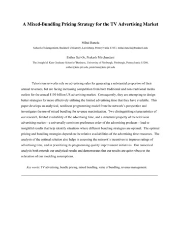
A Mixed-Bundling Pricing Strategy for the TV Advertising MarketMihai BanciuSchool of Management, Bucknell University, Lewisburg, Pennsylvania 17837, mihai.banciu@bucknell.eduEsther Gal-Or, Prakash MirchandaniThe Joseph M. Katz Graduate School of Business, University of Pittsburgh, Pittsburgh, Pennsylvania 15260,esther@katz.pitt.edu, pmirchan@katz.pitt.eduTelevision networks rely on advertising sales for generating a substantial proportion of theirannual revenues, but are facing increasing competition from both traditional and non-traditional mediaoutlets for the annual 150 billion US advertising market. Consequently, they are attempting to designbetter strategies for more effectively utilizing the limited advertising time that they have available. Thispaper develops an analytical, nonlinear programming model from the network’s perspective andinvestigates the use of mixed bundling for revenue maximization. Two distinguishing characteristics ofour research, limited availability of the advertising time, and a structural property of the televisionadvertising market—a universally consistent preference order of the advertising products—lead toinsightful results that help identify situations where different bundling strategies are optimal. The optimalpricing and bundling strategies depend on the relative availabilities of the advertising time resources. Theanalysis of the optimal solution also helps in assessing the network’s incentives to improve ratings ofadvertising time, and in prioritizing its programming quality improvement initiatives. Our numericalanalysis both extends our analytical results and demonstrates that our results are quite robust to therelaxation of our modeling assumptions.Key words: TV advertising, bundle pricing, mixed bundling, value of bundling, revenue management.
1. IntroductionAdvertising accounts for about two thirds of the total revenue1 for a typical television broadcast network.While the quality of the programming affects the ratings and thus the demand for television advertising,effective strategies for selling the advertising time are an important determinant of the broadcaster’srevenue. Determining such strategies is particularly important because the broadcaster’s availableadvertising time is limited either by competitive reasons (as in the US, where commercials account forroughly eight minutes for every 30 minute block of time) or by government regulations (as in theEuropean Union,2 where commercials are limited to at most 20 % of the total broadcast time). Moreover,the advertising time is a perishable resource; if it is not used for showing a revenue-generatingcommercial, the time and the corresponding potential revenue is lost forever.Broadcasters therefore use a multi-pronged strategy to capture revenues from the roughly 150billion dollar advertising market in the US.3 The market for selling television advertising time is split intotwo different parts: the upfront market, which accounts for about 60%-80% of airtime sold and takesplace in May every year, and the scatter market which takes place during the remainder of the year. Inthe first stage of their strategy, broadcast networks make decisions about how much advertising time tosell in the upfront market and how much to keep for the scatter market. On their part, clients purchaseadvertising time in bulk, guided by their medium-term advertising strategy, during the upfront market (atprices that may eventually turn out to be higher or lower than the scatter market prices). The scattermarket, on the other hand, allows advertisers to adopt a “wait-and-see” approach to verify the popularityof various network shows, and tailoring their decisions to match their short term advertising strategy.Our work develops revenue maximizing strategies as they apply to broadcast networks makingdecisions during the scatter market period. The broadcaster makes available for sale limited amounts ofadvertising time during different categories of daily viewing times. Advertisers value these categoriesdifferently because television audience size varies by the time of the day. In particular, evening time,called prime time, traditionally attracts the most viewers, and as such is deemed more valuable by theadvertisers, while the rest of the viewing time is referred to as non-prime time. A critical decision for the1Ad Revenue Down, CBS Posts Profit Drop of 52%. The New York Times, February 18, s/getDoc.do?language NL&type IM-PRESS&reference 20071112IPR1288332007 TNS media intelligence report (http://www.tns-mi.com/news/03252008.htm). Of this amount, televisionadvertising accounts for roughly 64 billion annually.2
broadcaster is how to price these products (that is, the advertising time sold in the different categories) atlevels that maximize revenue. Optimally aligning the prices with the advertiser’s willingness to payensures that the network neither leaves “money on the table,” nor uses the advertising resourceinefficiently. Moreover, ad hoc pricing can lead to improper market segmentation: advertisers with ahigher propensity to pay may end up buying a less expensive product. Likewise, some potentialadvertisers may be priced out of the market due to improper pricing, even though doing so may beunprofitable for the network. The broadcast network faces yet another decision which is based on anevaluation of the benefits of enhancing the programming quality. Improving quality requires effort (timeand money), but can lead to higher ratings. However, the impact of better quality on the network’sprofitability may be different depending on whether it relates to prime or to non prime time programming.The question that broadcasters need to answer is the amount of effort they should apply to improveprogramming quality.The complexity in the analysis for the situations described above gets amplified significantly ifthe network decides to use bundling—the strategy of combining several individual products for sale as apackage (Stigler, 1963). In this regard, the broadcaster has several options available (Adams and Yellen,1976): (i) pure components strategy, that is, offer for sale the different categories of advertising time asseparate items only; (ii) pure bundling strategy, that is, offer for sale advertising time from the differentcategories only as a package; and (iii) mixed bundling strategy, that is, offer for sale both the bundle andthe pure components. Mixed bundling offers an opportunity to the broadcaster to more precisely segmentthe market. However, as the number of constituent components increases, the number of bundles that wecan offer in a mixed-bundling strategy increases exponentially. As a consequence, the number of pricingrelationships that need to hold also increases exponentially. Specifically, the broadcaster needs to ensurethat the price of each bundle should be no more than the price of its constituent parts. Otherwise, theadvertiser can simply buy the constituent parts instead of the bundle (Schmalensee, 1984). If the numberof bundles is exponential, so is the number of such pricing constraints. To keep the problem tractable,and since our intent is to draw out qualitative managerial insights to help the broadcaster make decisionsregarding the available advertising time resources during the scatter market, we begin by assuming thatthe components each consist of one unit of prime and non-prime time respectively, and the bundleconsists of one unit each of the two components. We later show that under some situations these earlierresults apply with a simple recalibration of the units of measurement of the components. When thebundle composition can be chosen by the advertiser, one might consider potentially using an elegantapproach proposed by Hitt and Chen (2005). This approach, customized bundling, allows buyers tothemselves create for a fixed price idiosyncratic bundles of a specified cardinality from a larger set ofavailable items. Wu et al. (2008) use nonlinear programming to further explore the properties of3
customized bundling. The customized bundling approach is not needed for the equal proportionstelevision advertising case that we are considering; moreover, as we discuss later, we assume that theavailable resources are limited, and so the customized bundling model does not directly apply. Therefore,we focus on the seller (that is, the network broadcaster) creating and offering the bundle for sale.In the television advertising case (as opposed to other bundling situations), the two componentshave a fundamental structural relationship. Since viewership during prime time hours exceeds theviewership during non-prime time hours, all advertisers prefer to advertise during prime time as comparedto advertising during non-prime time hours. Therefore, the prime time product offered is more attractivethan the non-prime time product. This natural ordering of the advertising products offered by thebroadcaster implies that, given suitably low prices for the three products, all advertisers prefer the nonprime time product to no advertising, the prime time product to the non-prime time product, and thebundle to the prime time product. In the bundling context, this type of preference ordering between thecomponents does not always exist. Indeed, the traditional bundling literature has focused onindependently valued products (e.g., Adams and Yellen, 1976, Schmalensee, 1984, McAfee, McMillan,and Whinston, 1989, Bakos and Brynjolfsson, 1999) or assumed that the bundle consists of substitutableor complementary components (Venkatesh and Kamakura, 2003). Products are independently valued ifthe reservation price of the bundle is the sum of the reservation prices of the components. When therelationship is complementary, the reservation price of the bundle may exceed the sum of the reservationprices of its constituents (Guiltinan, 1987), and when the constituents are substitutable, the bundle’sreservation price may (though not necessarily) be lower than the sum of the reservation prices of the twoconstituents. (Marketers may still offer the bundle to exploit market segmentation benefits, and becausethe variable cost of the bundle may be a subadditive function of the component variable costs.)Substitutable products may (as in the case of a slower versus a faster computer system) or may not (as inthe case of Coke versus Pepsi, or a slower versus a faster automobile) be amenable to a universallyconsistent ordering. Regardless, independent and complementary products clearly lack the naturalordering that we see for television advertising, where all advertisers prefer prime time advertising to nonprime time advertising.This type of ordering in the advertisers’ preferences also exists in some other commerciallyimportant practical situations. Radio or news magazine advertising are obvious examples. Additionally,in internet advertising, advertisers prefer placing an advertisement on the front page of a website toplacing it on a lower ranking page. Billboard advertising also exhibits this relationship. Here, placing abillboard advertisement featured along an interstate highway is preferred to placing the sameadvertisement on a secondary road, where the exposure to the advertisement may be more limited. While4
in this paper we use television advertising as a prototypical example, our model and results apply to othersituations that exhibit the preference ordering. As we will see, this preference ordering in the productsleads to some counter-intuitive and insightful results.Another distinctive feature of our research concerns the total amounts of each type of advertisingtime available for sale. As is the case in practice, we assume that these amounts are limited, andinvestigate how the broadcast network’s decisions change as the availabilities change. In contrast,previous bundling literature has not modeled resource availabilities.This paper is organized as follows. Section 2 discusses our modeling assumptions and develops anonlinear pricing model for a bundling situation when the resources have limited availability. The outputfrom this model is a set of optimal product prices that automatically segments the market, andcorrespondingly sets the fraction of the market that is covered by each product. Advertisers decide on theproduct they wish to purchase based on the prices they are offered and their willingness to pay—which inturn depends on the “efficiency” with which they can generate revenues from viewers of theiradvertisements. In Section 3, assuming that the distribution of the advertiser’s efficiency parameter(which measures the effectiveness with which the advertiser translates viewers into revenue) is uniform,we analyze the properties of the optimal prices, and shadow prices. Interestingly, the tightness and therelative tightness of the advertising resources plays a pivotal role in not only affecting the product pricesbut also influencing whether or not to offer the bundle, and if the bundle is offered, the type of bundlingstrategy to adopt. When prime and non-prime time resource availability is unconstrained, the broadcasteroffers only the bundle. On the other hand, the broadcaster offers the bundle in conjunction with somecomponents only when there is “enough” prime and non-prime time advertising resource. We alsoanalyze the shadow prices of advertising resources, and evaluate how the broadcast network should focusits quality improvement efforts to improve total revenue. Due to bundling, the shadow price of the primetime resource (non-prime time resource) can decrease or remain the same even when its availability iskept unchanged but the availability of only the non-prime time resource (prime time resource) isincreased. Our analysis shows that when the relative availability of the two resources is comparable, italways makes more sense for the network to improve the ratings of the prime time product. This sectionalso explores the value of bundling. Section 4 relaxes two of the assumptions in our original model.Using specific instances from the Beta family of distributions to model the density function of advertiserefficiencies, we show numerically that the general nature of our conclusions is quite robust. We alsoinvestigate how to implement, and the impact of, a generalization of the definition of the bundle to allowfor an unequal mix its constituent components. Section 5 concludes the paper by identifying some futureresearch directions.5
2. The ModelA monopolist television broadcasting network, which we refer to as the broadcaster, considersoffering for sale on the scatter market its available advertising time, that is, its advertising inventory. Thisinventory is of two types: prime time and non-prime time. The availability of both of these inventories,which we interchangeably refer to also as resources, is fixed, with qP denoting the amount of advertisingtime available during prime time hours, and qN denoting the amount of advertising time available duringnon-prime time hours. The broadcaster’s objective is to maximize the total revenue it generates fromselling its inventory. As in the information goods situation in Bakos and Brynjolfsson (1999), we canassume that the variable costs of both resources is zero for our situation, and so maximizing the revenue isequivalent to maximizing the contribution. In order to do so, the broadcaster sells three productscorresponding to selling one unit of each of the two resources separately, and selling a bundle whichconsists of one unit of each resource.The market consists of advertisers interested in purchasing advertising time from the broadcaster.In line with the bundling literature (e.g., Adams and Yellen, 1976; Schmalensee, 1984), we assume that themarginal utility of a second unit of a product is zero for all advertisers. Advertisers have a strict orderingof their preferences: They consider advertising during non-prime time to be more desirable than notadvertising, prime time advertising to be more desirable than non-prime time advertising, and the bundlethat combines both prime and non-prime time advertising to be the most desirable. This preference is aconsequence of prime time ratings being higher than non-prime time ratings. We designate the ratings ofthe non-prime time, prime time, and the bundle options by α, β, and γ, respectively, where, 0 α β γ.We also assume that the relationship between the ratings is “concave” in nature, that is, α β γ. Thisassumption is reasonable because of diminishing returns seen in advertising settings: in this case, thesame individual might see an advertisement shown during both prime and non-prime time periods, and sothe rating of the bundle is less than the sum of the ratings of the prime and non-prime advertisements.Advertisers differ in their willingness to pay for the three advertising products due to their variedability to translate eyeballs into purchase decisions of viewers and the consequent profits. Advertiserswho are more successful in generating higher profits have a greater willingness to pay for the moredesirable products—which are also more expensive. We designate by the parameter t the intrinsicefficiency of an advertiser to generate profits out of advertisements, and assume that this efficiency isdistributed on the unit interval according to some probability density function f(t) and cumulativedistribution function F(t). The willingness to pay of an advertiser with efficiency t for an advertisement6
placed in time period i is thus equal to t ri, where ri is the rating of the ith product, i equal to prime, nonprime or the bundle.Given the above distribution of the efficiency parameter of advertisers and their willingness topay function, an optimal strategy for the broadcaster segments the population of advertisers into at mostfour groups as described in Figure 1, with the thresholds T*, T**, and T*** demarcating the differentmarket segments.4 With this strategy, advertisers in the highest range of efficiency parameters (interval[T*, 1]) choose to purchase the bundle. Those in the second highest range of efficiency parameters(interval [T**, T*)) choose to advertise during prime-time. Those in the third highest range (interval[T***, T**)) choose the non-prime product, and those in the lowest range refrain from advertisingaltogether. An interval of zero length implies that it is not optimal for the broadcaster to offer thecorresponding product. The values of the threshold parameters T*, T**, and T*** are determined toguarantee that the advertiser located at a given threshold level is indifferent between the two choicesmade by the advertisers in the two adjacent intervals separated by this threshold parameter.Figure 1. Market segmentationTo set up the model we define the selling prices for the bundle, prime, and non-prime products bypB, pP and pN, respectively. The revenue optimization with mixed bundling model (ROMB), from thebroadcaster’s perspective, is:[ROMB]1T*T **TTTmax π pB * f (t )dt pP ** f (t )dt pN *** f (t )dtpB , pP , p N 0(1)subject to:pB pP pN ,4(2)The willingness to pay function satisfies the “single crossing property” and therefore facilitates segmentation andguarantees the uniqueness, as well as the monotonicity (0 T*** T** T* 1) of the thresholds.7
1 1T*T*T*f (t )dt ** f (t )dt qP , andTT **f (t )dt *** f (t )dt qN .T(3)(4)The broadcaster’s revenue from a market segment equals its size multiplied by the price of theproduct it corresponds to; the total revenue, π, in the objective function (1) is the sum of the revenuesfrom each of the three segments that the broadcaster serves. Constraint (2), the “price-arbitrage”constraint, prevents arbitrage opportunities for an advertiser to compose a bundle by separately buying aprime and a non-prime time products separately.5 Constraints (3) and (4) model the limited prime andnon-prime time available.Advertisers self-select their purchases (or they may decide to not purchase any of the offeredproducts) based on their willingness to pay and the product prices. (See Moorthy, 1984, for an analysis ofself-selection based market segmentation.) Consider the difference between an advertiser’s willingness topay and the price of the product he6 purchases. This difference equals the premium the advertiser derivesfrom the purchase. An advertiser will purchase a product only if his premium is nonnegative. Moreover,an advertiser will be indifferent, say, between buying only prime time and buying a bundle consisting ofprime and non-prime time, if he extracts the same premium from either purchase. The followingrelationships between the purchasing premiums are invariant boundary conditions, regardless of theefficiency distribution f(t).γ T * pB β T * pP T * β T ** pP α T ** pN T ** α T *** pN 0 T *** pB p P,γ β(5)pP p N, andβ α(6)pNα.(7)Notice that the non-negativity of the thresholds implies5pP pB , and(8)p N pP .(9)Unless a systematic secondary market exists, an intermediary cannot purchase a bundle and then sell itscomponents individually at a profit.6Where necessary, we use masculine gender for the advertiser and feminine gender for the broadcaster.8
Moreover, it is easy to see that pN, as well as the premium for customers in each of the three categories, isnonnegative.Before we analyze the situations that arise when at least one of the capacity constraints is binding,Proposition 1 considers the case when neither capacity constraint is binding. Appendix I gives the proofof this and all subsequent results.Proposition 1. If the prime and non-prime resource availability is sufficiently high, the optimal strategyfor the broadcaster is pure bundling. The corresponding optimal threshold is the fixed point of the(reciprocal of the hazard rate function of the distribution of advertisers, that is, T * 1 F (T * )) f (T ) .*The following corollary uses Markov’s inequality to establish an upper bound on the optimalrevenue when the problem is not constrained by the inventory availability.Corollary 2. An upper bound on the broadcaster’s total revenue π is γ E [T ] , where E [T ] is the expectedvalue of the efficiency, t. The actual revenue collected under the pure bundling strategy is(γ 1 F (T * )) f (T ) .2*The result in Proposition 1 seems to contradict previous bundling literature (for example,Schmalensee, 1984, McAfee, McMillan, Whinston, 1989) which demonstrates that the mixed bundlingstrategy weakly dominates both the pure bundling and pure components strategies. However, a criticaldifference between our model and previous work is that the advertisers have a common preferred orderingof the three products. In contrast, the previous research stream does not assume any such ordering of theproducts. Since the bundle is the most desirable option for every advertiser, the broadcaster offers onlythe bundle when the available prime and non-prime advertising time is unconstrained. This unconstrainedcase is unlikely to arise in reality, since all broadcasters are usually heavily constrained by the prime timeresource availability.In the next section we derive the analytical solution of the constrained optimization problemunder the simplifying assumption that the efficiency parameter of advertisers is uniformly distributed. InSection 4, we extend the results numerically using a Beta Distribution.3. Revenue Maximizing Strategies when Capacity is BindingClearly, the capacity constraints in the ROMB model play a significant role in determining thebroadcaster’s optimal strategy. Particularly, the relative scarcity of the two resources, prime time andnon-prime time, is the main driver of the analysis. In the television advertising market, the prime time9
resource availability constraint (3) is far more likely to be binding than the non-prime time resourceavailability constraint (4). Prime time on television is usually the slot from 8:00 pm until 11:00 pmMonday to Saturday, and 7:00 pm to 11:00 pm on Sunday. Hence, the ratio of prime to non-prime timeavailability is about 1:8 (or 1:6 on Sunday). In other media markets, the relative scarcity of the non-primetime constraint may also become an issue. For instance, in the billboard advertising market, the “nonprime time” resource is the limited availability of billboards on secondary roads (which are less traveled),whereas the “prime time” is the extensive availability of billboard advertisement space on major roads(which have more travelers). In such a market, it is the “non-prime time” capacity that is more likely tobe binding. Finally, in internet advertising both types of capacity constraints may be binding. Eachwebsite has limited space for banner advertisements irrespective of whether it is the front page (“primetime”) or a secondary page (“non-prime time”). In this section, we specify the distribution of theefficiency parameter of advertisers to be uniform and identify the impact of the two capacity constraintson the type of strategy followed by the broadcaster. We find that the following strategies can arise as theoptimal solution of ROMB: no bundle is offered, that is, the pure components strategy, PC; only thebundle is offered, that is, the pure bundling strategy, PB; the bundle, as well as each separate time productis offered, that is, the full spectrum mixed bundling strategy, MBPN; the bundle and the prime timeproduct are offered, that is, the partial spectrum mixed bundling strategy, MBP; the bundle and the nonprime time product are offered, that is, the partial spectrum mixed bundling strategy, MBN. Throughoutthe remainder of the paper we will refer to these abbreviations.In our derivations, we will demonstrate that the optimal strategy critically depends upon therelative availability of qP and qN. We will show that, for instance, that the MBN strategy is optimal whenqP is scarce relative to qN, and the MBP strategy arises in the opposite case. The MBPN strategy is theoptimal strategy when the ratio of qP to qN is close to one, but they are both sufficiently large.We will also show that the characterization of the solution when the partial spectrum mixedbundling strategies (MBP or MBN) are optimal is further contingent upon the overall availability of themore abundant resource. Specifically, even though the strategy itself, say MBP, remains the same, thesolution characteristics (product prices and the shadow prices of the resources) depend on whether qP isless than or greater than a half. Similarly, the characteristics of the solution corresponding to MBNdepend on whether qN is less than or greater than a half. To distinguish between these two cases, wedesignate by MBP and MBP the partial spectrum mixed bundling strategies when qP is greater than andwhen qP is less than a half, respectively. We define the subcategories MBN and MBN of MBN in asimilar manner depending on the availability of qN.10
Figure 2 depicts the regions corresponding to the various strategies that we discussed above. Forthe uniform distribution, the unconstrained solution that we described in Section 2 arises when qP and qNare both at least a half. In this case, at the optimal solution, the broadcaster never sells more than anaggregate quantity of one, split equally between the prime and non-prime advertising times. To depict theconstrained solution, therefore, in Figure 2, we restrict attention only to the case when qP qN 1. Theunconstrained solution in the figure is designated by the point, PB, where qP qN ½. The boundariesfor the regions in Figure 2 will be explained in detail once the solution to model ROMB is derived.1121 γ β 22α1 γ β11 22α2Figure 2. Representation of the optimal strategiesReplacing the general distribution by a uniform distribution in the model ROMB yields thefollowing model, which we refer to as ROMB U. [ROMB U] max π pB 1 p B pPγ β p B pP p P p N pP β α γ β pP p N p N pN α β α (10) subject to:pB ( pP pN ) 0,1 1 pP p N qP , andβ αp B p P pP p N p N qN .γ ββ αα(11)(12)(13)11
It is easy to see that the solution to the unconstrained case (when qP ½ and qN ½) is pB γ/2,pP β/2, and pN α/2. This solution guarantees that only pure bundling arises since T* T** T*** ½, and the broadcaster’s revenues are γ/4. Note that this solution also guarantees that the arbitrageconstraint pB is pP pN is satisfied since γ α β by the concavity assumption.3.1. Characterization of the Different StrategiesWe now discuss the characterization of the constrained case. Proposition 3 describes theboundaries of the regions corresponding to the different strategies depicted in Figure 2, and Propositions3 and 4 derive the optimal product and the shadow prices, respectively.Proposition 3. The optimal strategies as a function of the availability of qP and qN are as follows:(i)The pure component strategy, PC, is optimal if0 q N qP (ii)1 γ β .22αThe full spectrum mixed bundling strategy, MBPN, is optimal ifγ β 1 2q Nα .1 2qP γ βα(iii)The partial spectrum mixed bundling strategies, MBN and MBN , are optimal if 0 qP ½,anda.1 2qN γ β1 and qN for MBN ,1 2q P2αb. qN (iv)1for MBN .2The partial spectrum mixed bundling strategies, MBP and MBP , are optimal if 0 qN ½anda.1 2q N1α and qP for MBP ,1 2qP γ β2b. qP (v)1for MBP .2The pure bundling strategy, PB, is optimal at a single point qP qN ½.According to Proposition 3 when the available aggregate capacity is small (lower than1 γ β 22α), the broadcaster follows a pure component strategy where each advertiser can choose betweenadvertising on prime time or on non-prime time but not both. Offering the bundle is suboptimal in thiscase given the extreme scarcity of the advertising time availability. When the aggregat
the pure components. Mixed bundling offers an opportunity to the broadcaster to more precisely segment the market. However, as the number of constituent components increases, the number of bundles that we can offer in a mixed-bundling strategy increases exponentially. As a consequence, the number of pricing