Transcription
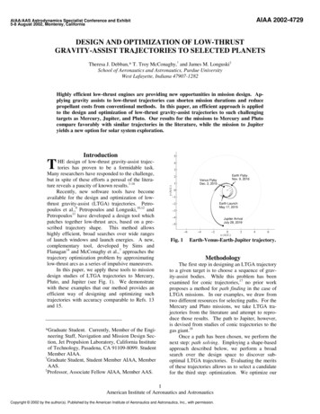
AIAA 2002-4729AIAA/AAS Astrodynamics Specialist Conference and Exhibit5-8 August 2002, Monterey, CaliforniaDESIGN AND OPTIMIZATION OF LOW-THRUSTGRAVITY-ASSIST TRAJECTORIES TO SELECTED PLANETSTheresa J. Debban,* T. Troy McConaghy,† and James M. Longuski‡School of Aeronautics and Astronautics, Purdue UniversityWest Lafayette, Indiana 47907-1282Highly efficient low-thrust engines are providing new opportunities in mission design. Applying gravity assists to low-thrust trajectories can shorten mission durations and reducepropellant costs from conventional methods. In this paper, an efficient approach is appliedto the design and optimization of low-thrust gravity-assist trajectories to such challengingtargets as Mercury, Jupiter, and Pluto. Our results for the missions to Mercury and Plutocompare favorably with similar trajectories in the literature, while the mission to Jupiteryields a new option for solar system exploration.Introduction5T*Graduate Student. Currently, Member of the Engineering Staff, Navigation and Mission Design Section, Jet Propulsion Laboratory, California Instituteof Technology, Pasadena, CA 91109-8099. StudentMember AIAA.†Graduate Student, Student Member AIAA, MemberAAS.‡Professor, Associate Fellow AIAA, Member AAS.43Earth FlybyNov. 9, 20162Venus FlybyDec. 2, 20151y (A.U.)HE design of low-thrust gravity-assist trajectories has proven to be a formidable task.Many researchers have responded to the challenge,but in spite of these efforts a perusal of the literature reveals a paucity of known results.1-16Recently, new software tools have becomeavailable for the design and optimization of lowthrust gravity-assist (LTGA) trajectories. Petropoulos et al.,9 Petropoulos and Longuski,10,12 andPetropoulos11 have developed a design tool whichpatches together low-thrust arcs, based on a prescribed trajectory shape. This method allowshighly efficient, broad searches over wide rangesof launch windows and launch energies. A new,complementary tool, developed by Sims andFlanagan14 and McConaghy et al.,7 approaches thetrajectory optimization problem by approximatinglow-thrust arcs as a series of impulsive maneuvers.In this paper, we apply these tools to missiondesign studies of LTGA trajectories to Mercury,Pluto, and Jupiter (see Fig. 1). We demonstratewith these examples that our method provides anefficient way of designing and optimizing suchtrajectories with accuracy comparable to Refs. 13and 15.0 1Earth LaunchMay 17, 2015 2 3 4Jupiter ArrivalJuly 28, 2019 5 6Fig. 1 4 20x (A.U.)246Earth-Venus-Earth-Jupiter trajectory.MethodologyThe first step in designing an LTGA trajectoryto a given target is to choose a sequence of gravity-assist bodies. While this problem has beenexamined for conic trajectories,17 no prior workproposes a method for path finding in the case ofLTGA missions. In our examples, we draw fromtwo different resources for selecting paths. For theMercury and Pluto missions, we take LTGA trajectories from the literature and attempt to reproduce those results. The path to Jupiter, however,is devised from studies of conic trajectories to thegas giant.18Once a path has been chosen, we perform thenext step: path solving. Employing a shape-basedapproach described below, we perform a broadsearch over the design space to discover suboptimal LTGA trajectories. Evaluating the meritsof these trajectories allows us to select a candidatefor the third step: optimization. We optimize our1American Institute of Aeronautics and AstronauticsCopyright 2002 by the author(s). Published by the American Institute of Aeronautics and Astronautics, Inc., with permission.
trajectories to maximize the final spacecraft mass,which in turn may increase the scientific value of amission.Broad SearchWe desire a computationally quick and efficient method of searching a broad range of launchdates and energies. For this process, we use a twobody patched-arc model. These arcs can be eithercoast only, thrust only, or a combination of thetwo. The coast arcs are standard Keplerian conicsections. The thrust arcs, however, are representedby exponential sinusoids9 which are geometriccurves parameterized in polar coordinates (r, θ ) asr k 0 exp[k1 sin( k 2θ φ )](1)where k0, k1, k2, and φ are constants defining theshape and, consequently, the acceleration levels ofthe arc. These exponential sinusoids can bepropagated analytically, which eliminates the needfor time-consuming numerical propagation. Themathematical and algorithmic details are workedout in Refs. 9-12, and the algorithms are implemented as an extension of the Satellite Tour Design Program (STOUR).19To evaluate the many candidate trajectoriesfound by STOUR, we employ a cost function thatcomputes the total propellant mass fraction due tothe launch energy, thrust-arc propellant, and arrival V (if a rendezvous is desired).7 Tsiolkovksy’s rocket equation is used to account for thedeparture and arrival energies.20,21 For the launchV ( V1 in Eq. 2), we use a specific impulse of350 seconds (Isp1) to represent a chemical launchvehicle. A low-thrust specific impulse (Isp2) of3000 seconds is applied to the arrival V ( V2)because we assume that the low-thrust arcs willremove any excess velocity in rendezvous missions. Finally, the thrust-arc propellant mass fraction given by STOUR (pmf) yields the total propellant mass fraction (tmf): V1 exp V 2t mf 1 (1 p mf ) exp gI sp1 gI sp 2 To reduce mission costs, the minimum totalpropellant mass fraction is desired. Since time offlight is not included in the cost function, it mustbe evaluated in conjunction with the total propellant mass fraction. This, of course, requires engineering judgment and a balancing of factors for aparticular mission. It is up to the mission designerto judiciously select the most promising trajectories to use as initial guesses for optimization.OptimizationOnce good candidate trajectories are found,we optimize them with the direct method developed by Sims and Flanagan.14 Our software,GALLOP (Gravity-Assist Low-thrust Local Optimization Program),7 maximizes the final massof the spacecraft. The essential features and assumptions of GALLOP are as follows (see Fig.2). The trajectory is divided into legs betweenthe bodies of the mission (e.g. an EarthMars leg).Each leg is subdivided into many shortequal-duration segments (e.g. eight-daysegments).The thrusting on each segment is modeledby an impulsive V at the midpoint of thesegment. The spacecraft coasts on a conicarc between the V impulses.The first part of each leg is propagated forward to a matchpoint, and the last part ispropagated backward to the matchpoint.Gravity-assist maneuvers are modeled asinstantaneous rotations of the V .The optimization variables include thelaunch V , the V on the segments, the launch,MatchpointPlanet or target bodySegment midpointImpulsive VSegment boundary (2) For flyby missions, V2 0. While Eq. 2 is only anapproximation of the true propellant costs, itserves quite adequately to reduce the candidatetrajectories to a manageable number among themyriad (up to tens of thousands) of possibilitiesproduced by STOUR.Fig. 2LTGA trajectory model (after Simsand Flanagan14).2American Institute of Aeronautics and Astronautics
flyby and encounter dates, the flyby altitudes, theflyby B-plane angles, the spacecraft mass at eachbody, and the incoming velocity at each body.The initial spacecraft mass can also be determined with a launch vehicle model so that theinjected mass is dependent upon the launch V .There are also two sets of constraint functions. One set ensures that the V impulses canbe implemented with the available power. Theother set enforces continuity of position, velocity, and spacecraft mass across the matchpoints(see Fig. 2). The optimizer uses a sequentialquadratic programming algorithm to maximizethe final mass of the spacecraft subject to theseconstraints.7Reference 7 provides more details on thebroad search and optimization procedures. Ourmethod is also demonstrated on simple examplesin Ref. 7. In this paper, we tackle more challenging problems using more mature versions of oursoftware.Optimized TrajectoriesThe success of our approach is illustrated inthe following examples. The first two, missionsto Mercury and to Pluto, are attempts to match orimprove upon optimized results in the literature.The last example is a mission to Jupiter that wedeveloped with no a priori knowledge of whatthe final, optimal result might be. In this case,we demonstrate the efficiency of our method byassessing the level of (computational and human)effort required to design and optimize the trajectory.Earth-Venus-Mercury RendezvousRendezvous missions to Mercury are particularly challenging for several reasons, including its proximity to the sun and the eccentricityand inclination of Mercury’s orbit. Even assuming circular, coplanar orbits of both Earth andMercury, a Hohmann transfer requires a launchV of at least 7.5 km/s, and the resulting arrivalV magnitudes can be as high as 9.6 km/s.22 Theuse of standard, chemical propulsion systems forremoving this excess velocity on arrival can beprohibitive. Taking into account Mercury’shighly eccentric and inclined orbit makes therendezvous task even more daunting.LTGA techniques offer low launch energieswhile Solar Electric Propulsion (SEP) systemscan efficiently eliminate the arrival V . Sauerincorporates a Venus flyby en route to Mercuryto further facilitate the mission.13 Sauer’s opti-mized trajectory (using SEPTOP, an indirectmethod) has approximately 6.5 total revolutionsaround the sun, 5.75 of which occur on the Venus-Mercury leg of the mission. The “spiraling”in this trajectory is necessitated by the limitedthrusting capability of a single SEP engine.7,13,14We began our quest for an initial guess forGALLOP by performing a search in STOUR.We searched over a five-year period that included the launch date in Sauer’s optimized trajectory.13 Our Earth-Venus trajectory leg was apure thrust leg, while the Venus-Mercury legwas a coast-thrust leg. We allowed the spacecraft to coast for more than one full revolutionbefore starting to thrust at 0.68 AU. The coasttime allows the exponential sinusoid geometry tobe better aligned with the geometry of Mercury’sorbit.11 The additional coast revolution also provides GALLOP with more time to thrust.Initially, we based our trajectory selectionon the lowest total propellant mass fraction. Ourattempts to optimize this case in GALLOP, however, were hindered by the thrust limitations ofone SEP engine. Our trajectory had just underfive total revolutions around the sun with onlyfour complete revolutions on the Venus-Mercuryleg. Given this trajectory profile, we concludedthat the spacecraft could not provide sufficientacceleration to rendezvous with Mercury.Reviewing our STOUR results, we sought acase with a higher number of Venus-Mercuryrevolutions. We limited our search to launch V magnitudes within 1 km/s of Sauer’s value (of2.3 km/s).13 By taking the trajectory with themaximum number of Venus-Mercury revolutionsin this launch V range, we obtained a casewhose time of flight is only three days longerthan Sauer’s and whose launch date is less thanfour weeks earlier (see Table 1). In addition, thistrajectory has 5.5 Venus-Mercury revolutions,which is only a quarter of a revolution less thanSauer’s case.With this initial guess, we were able to successfully optimize this trajectory in GALLOP.The initial launch mass is dependent upon thelaunch V magnitude via a Delta 7326 launchvehicle model. This is the Medlite Delta used bySauer.13 Sauer, however, uses a 10% launchmargin so that the initial mass is only 90% ofthat available for a given launch V . Our modeluses the full 100% launch mass, so we expectour final results to be somewhat different thanthose of Ref. 13.Figure 3 shows the final, optimized trajectory. Each dot represents the midpoint of the3American Institute of Aeronautics and Astronautics
Table 1 Earth-Venus-Mercury rendezvous trajectorySTOURGALLOPEarth launch dateAug. 2, 2002Aug. 13, 20023.00 km/s1.93 km/sLaunch V Delta 7326Launch vehicleN/AaInitial massN/Aa603 kgEarth-Venus time of flight (TOF)184 days198 daysVenus flyby dateFeb. 2, 2003Feb. 27, 2003Venus flyby altitude86,982 km200 kmbVenus-Mercury TOF667 days655 daysMercury arrival dateNov. 30, 2004Dec. 13, 2004Total TOF851 days853 daysFinal massN/Aa416 kgPropellant mass fraction0.5260.310Sauer13Aug. 27, 20022.31 km/sDelta 7326521 kg185 daysFeb. 28, 2003NRc663 daysDec. 22, 2004848 days377 kg0.276aNot applicable.Flyby at altitude lower limit.cNot reported.bsegments described in the optimization section(see Fig. 2). The line emanating from a givendot shows the direction and relative magnitudeof the thrust vector on that segment. In this case,each Earth-Venus segment represents 8.25 dayswhile each Venus-Mercury segment is only 3.90days. Our “rule of thumb” for selecting thenumber of segments on a given leg is to aim foran eight-day segment-length because this valuehas provided good results without necessitatingan excessive number of variables.7 (A largenumber of variables can slow GALLOP’s computation time.) We decided, however, to usesegments of about four days for the VenusMercury leg because of the high angular velocities close to the sun. Eight days is approximately9% of a Mercurian year whereas the sameamount of time is only about 2% of Earth’s year.The shorter, four-day segments provide higherfidelity for the spiraling trajectory leg.10.80.6Mercury ArrivalDec. 13, 20040.4y (A.U.)0.20 0.2 0.4 0.6Venus FlybyFeb. 27, 2003Earth LaunchAug. 13, 2002 0.8 1 1 0.50x (A.U.)0.5Figure 3 also shows significant coast periodsthrough each apoapsis of the Venus-Mercury leg.These coast periods are also evident in Sauer’strajectory.13 This close correspondence in thrustprofile suggests that both methods have found anoptimal solution.Table 1 shows good agreement between theresults obtained from STOUR, GALLOP, andSauer. We attribute STOUR’s high propellantmass fraction to the trajectory shape imposed bythe exponential sinusoid. It is expected that anoptimized solution will improve upon this shape.We also note that the final mass from GALLOP is actually higher than Sauer’s, but this isoffset by GALLOP’s higher propellant massfraction. While Sauer’s trajectory has a higherlaunch V magnitude, GALLOP uses morethrust on the Earth-Venus leg. Sauer’s optimaltrajectory coasts for approximately the last thirdof the Earth-Venus leg, whereas the GALLOPtrajectory has only a short coast phase on that leg(see Fig. 3). In a sense, GALLOP trades theadditional launch energy for more SEP enginethrust time. These differences can account forGALLOP’s earlier launch date. GALLOP needsthe additional thrusting time to achieve the necessary change in energy for the Venus flyby(which occurs only 1 day earlier than the Venusflyby in Sauer’s trajectory). We believe thatmany of the differences in the launch V magnitude, initial and final masses, propellant massfraction, dates, and Earth-Venus thrust profileare due to the 10% launch vehicle margin inSEPTOP.1Fig. 3 Earth-Venus-Mercury trajectory.4American Institute of Aeronautics and Astronautics
Earth-Venus-Jupiter-Pluto FlybyMissions to Pluto present a different set ofobstacles to mission designers, although the inclination and eccentricity of Pluto’s orbit areagain responsible for some of these difficulties.The chief obstacle, however, is Pluto’s distancefrom the sun. Because the solar power availableat large distances from the sun is not enough tooperate the SEP engines, LTGA trajectories using SEP cannot provide a rendezvous with Pluto.Therefore, the trajectory we present in this paperhas a Pluto flyby.The search for a trajectory to Pluto beganwith a trajectory presented by Williams andCoverstone-Carroll.15 Using the VARITOP optimization software, they optimized an LTGAmission to Pluto via gravity assists from Venusand Jupiter with a launch in June 2004.We implemented this path (Earth-VenusJupiter-Pluto) in STOUR to find an initial guessfor our optimizer. Unfortunately, STOUR couldonly produce results with long times of flight inthe vicinity of the Williams and CoverstoneCarroll launch date because the exponential sinusoid is better at approximating trajectory arcswith low eccentricities. Trajectories to Plutowith reasonably short flight times, however, generally require high flyby velocities at Jupiteroften resulting in heliocentric escape.22 Although Ref. 22 did not address LTGA trajecto-ries, the SEP engine’s inability to thrust as farout as Jupiter means that a high V at Jupiter isrequired in our case, as well.We accepted long flight times in STOURwith the understanding that the exponential sinusoid would not provide optimal energy increaseson the Venus-Jupiter leg. In fact, the STOURorbits from Jupiter to Pluto were actually elliptical. This accounts for the lengthy time of flight(TOF) of 6177 days on that leg in our chosentrajectory (see Table 2). STOUR managed tofind trajectories with launch dates very close tothose in Ref. 15, however. The minimum costfunction trajectory in STOUR launches only twoweeks prior to the trajectory in Ref. 15 and wasselected as our initial guess for GALLOP.With the STOUR initial guess, we were ableto achieve an optimal solution in GALLOP usinga Delta 7326 launch vehicle model to determinethe initial mass (see Fig. 4). We note that anyoptimal result obtained in this case is dependentupon the bounds set on the Pluto arrival date.The final spacecraft mass increases as the arrivaldate is allowed to be pushed later by the optimizer. We accepted the 8.9 year TOF as a good,comparable result to the Williams and Coverstone-Carroll case (see Table 2).15It should be noted that there are significantdifferences between our optimal result and thatin Ref. 15. First of all, GALLOP uses a singleTable 2 Earth-Venus-Jupiter-Pluto flyby trajectorySTOURGALLOPVARITOP15Earth launch dateMay 25, 2004May 17, 2004June 8, 20047.5 km/s5.28 km/s5.73 km/sLaunch V Delta 7326Delta 7925Launch vehicleN/AaInitial massN/Aa331.9 kg562.3 kgEarth-Venus TOF96 days126 days115 daysVenus flyby dateAug. 28, 2004Sept. 20, 2004Oct. 1, 2004Venus flyby altitude5197 km200 kmb300 kmVenus-Jupiter TOF659 days503 days471 dayscJupiter flyby dateJune 18, 2006Feb. 5, 2006Jan. 2006Jupiter flyby altitude4.5 Rjd7.2 Rjd7.2 RjdJupiter-Pluto TOF6177 days2614 days2616 daysePluto arrival dateMay 17, 2024Apr. 3, 2013Mar. 20135.9 km/s17.2 km/sNRfArrival V Total TOF19 years8.9 years8.8 yearsFinal massN/Aa231.0 kg420.2 kgPropellant mass fraction0.3530.3040.253aNot applicable.Flyby at altitude lower limit.Estimated from Oct. 1, 2004 to Jan. 15, 2006. Specific Jupiter flyby date not reported in Ref. 15.dJovian radii. 1 Rj 71,492 km.eEstimated from Jan. 15, 2006 to Mar. 15, 2013. Specific Jupiter and Pluto flyby dates not reported in Ref. 15.fNot reported.bc5American Institute of Aeronautics and Astronautics
2Venus flybySept. 20, 20041y (A.U.)0 1Earth launchMay 17, 2004 2 3 4 6Jupiter flybyFeb. 5, 2006To PlutoArrive April 3, 2013 5Fig. 4 4 3 2x (A.U.) 1012Earth-Venus-Jupiter-Pluto trajectory.SEP engine model. Second, we assumed thesolar arrays could provide 10 kW of power at 1AU. We also implemented the relatively smallDelta 7326 launch vehicle model. A largerlaunch vehicle would have injected more massfor the same launch V , but the single SEP engine would not have been able to provide sufficient thrust on such a large spacecraft.Williams and Coverstone-Carroll, on theother hand, use three SEP engines and the morepowerful Delta 7925 launch vehicle.15 As withthe trajectory to Mercury, this launch model includes a contingency margin – 14% in this case.The solar array power for their trajectory,though, was only 6 kW.15 The lower solar arraypower means that the available thrust begins todecrease closer to the sun than with the 10 kWwe assumed in GALLOP.Because of the differences in launch vehicle,launch vehicle margin, number of SEP thrusters,and solar arrays it is difficult to draw any conclusions about the superiority of the either theGALLOP or VARITOP results. What our trajectory does show, however, is that it is possible toreach Pluto in less than nine years with a modestlaunch vehicle by employing LTGA techniques.Earth-Venus-Earth-Jupiter FlybyFor our final trajectory we opted for a different approach to the path-finding problem.Instead of looking for LTGA paths already developed, we investigated paths previously developed for conic trajectories.18 In particular, welooked for trajectories that required significantmid-course V maneuvers because we assumedthat the SEP engine’s capabilities would removethe need for such events.Having selected Jupiter as our target body,we turned to work performed by Petropoulos etal.18 for gravity-assist missions to Jupiter. Inorder to design and optimize a trajectory thatcould be flown before the end of the next decade,we looked for promising trajectories that launchin the years ranging from 2010 to 2020. Ref. 18suggests that gravity assists from Venus andEarth can provide short flight times at the expense of a mid-course maneuver. We thereforechose to search for trajectories with the EarthVenus-Earth-Jupiter (EVEJ) path in STOUR.STOUR searched launch dates from January1, 2009 to January 1, 2021 at a 10-day step. Thesearch also included launch V values of 1.0km/s to 4.5 km/s at a 0.5 km/s step. The arcsfrom Earth to Venus and Venus to Earth werepure thrust arcs. The Earth-Jupiter leg of themission thrusted out to 5.0 AU where it switchedto a coast arc. Because of the minimum powerrequirements of the SEP engine, it is unable tothrust past approximately 4.7 AU.7 We allowSTOUR to thrust a little longer to compensatefor the sub-optimality of the exponential sinusoidshape.Figure 5 shows the results of this STOURsearch. This figure is a plot of the total flybypropellant mass fraction (tmf in Eq. 2 with V2 0)versus launch date. Because over 16,000 trajectories resulted from this search, we use this cost6American Institute of Aeronautics and Astronautics
0.90.85Total Propellant Mass Fraction0.80.750.70.650.60.552/3/20086/17/2009 10/30/2010 3/13/2012 7/26/2013 12/8/2014 4/21/20169/3/20171/16/2019 5/30/2020 10/12/20210.52454500 2455000 2455500 2456000 2456500 2457000 2457500 2458000 2458500 2459000 2459500Launch DateFig. 5Earth-Venus-Earth-Jupiter flyby cost function.function to help determine which regions of thedesign space are the most promising.Since we desire a trajectory with a low TOF,we do not simply select the trajectory with thelowest total propellant mass fraction. In addition, we consider the accelerations on each trajectory. STOUR computes the maximum andaverage acceleration values on each trajectory toindicate the amount of thrust needed to maintainthe exponential sinusoid shape. Since we assume a single thruster in GALLOP, we generallyopt for STOUR trajectories with low accelerationvalues. For the EVEJ case, the trajectories withlow cost functions (in Fig. 5) that launch shortlyafter Dec. 8, 2014 stand out as having both shortTOFs and low accelerations. Performing a morerefined, one-day step search over launch datesfrom Jan. 1, 2015 to Aug. 1, 2015 resulted in theSTOUR initial guess shown in Table 3.Using this STOUR guess, GALLOP obtained an optimal solution launching only oneweek later than the STOUR trajectory. Figures 1and 6 also show the thrust profile from theGALLOP result. This thrust profile is plotted inFig. 7 as the V magnitude on each segment(illustrated in Fig. 2). The maximum possible V magnitude on a given segment is dependenton three main factors: 1) the amount of time represented by a given segment, 2) the mass of thespacecraft on that segment, and 3) the distancefrom the sun.The first and third legs of the trajectory havehigher V magnitudes because more days arerepresented by these segments. The Earth-Venusand Earth-Jupiter legs have approximately 12day segments, whereas the Venus-Earth leg hassegments of about 8 days. The leg lengths aredifferent for two reasons. The first is that longersegments were used on the Earth-Jupiter leg because of the lower velocities at this distance fromthe sun. Second, GALLOP has the freedom tochange the flyby dates but not alter the numberof segments on each leg. The Venus flyby datewas moved so much later than the STOUR initialguess that the segments lengthened from justunder eight days to over twelve days.The maximum V available increasesthroughout the first leg and the beginning of thethird leg because the mass decreases as propellant is expelled (see Fig. 7). While the thrust is7American Institute of Aeronautics and Astronautics
Table 3 Earth-Venus-Earth-Jupiter flyby trajectorySTOURGALLOPMystic23Earth launch dateMay 9, 2015May 17, 2015May 16, 20152.0 km/s1.80 km/s1.78 km/sLaunch V Delta 7326Delta 7326Launch vehicleN/AaInitial massN/Aa609.6 kg610.9 kgEarth-Venus TOF119 days199 days200 daysVenus flyby dateSept. 5, 2015Dec. 2, 2015Dec. 2, 2015Venus flyby altitude4481 km200 kmb670 kmVenus-Earth TOF345 days343 days342 daysEarth flyby dateAug. 15, 2016Nov. 9, 2016Nov. 8, 2015Earth flyby altitude4219 km300 kmb300 kmbEarth-Jupiter TOF1027 days991 days966 daysJupiter arrival dateJune 8, 2019July 28, 2019July 2, 20195.97 km/s5.81 km/s5.88 km/sArrival V Total TOF1491 days, 4.1 years1533 days, 4.2 years1508 days, 4.1 years537.9 kg538.7 kgFinal massN/AaPropellant mass fraction0.4850.1180.118abNot applicable.Flyby at altitude lower limit.constant over these periods, the lower spacecraftmass on successive segments means a greater V is imparted by this thrust.The third factor controlling the maximumavailable thrust is the distance from the sun. Wemodel SEP engines that need a minimum amountof power to operate. (Solar array power is proportional to the inverse-square of the radius fromthe sun.) While there is sufficient power to operate at maximum thrust well past Mars’ orbit, atabout 2.2 AU the thrust levels drop off becauseof the loss of power, as can be seen in Fig. 7.Figure 7 also shows that while the VenusEarth STOUR leg was a pure thrust leg, GALLOP made that leg a pure coast arc. Furthermore, GALLOP cut off the thrust on the Earth-0.21.5Earth FlybyNov. 9, 2016Venus FlybyDelta V Magnitude (km/s)y (A.U.)0 0.5To Jupiter ArrivalJuly 28, 2019Fig. 6 1.5 10.140.120.10.080.060.04Earth LaunchMay 17, 2015 2Power availability constraintSolutionFlyby0.160.5 1.5Earth Flyby0.18Venus FlybyDec. 2, 20151 1Jupiter leg at about 1.6 AU as opposed the 5.0AU cut-off in STOUR. By moving the Venusand Earth flyby dates several months later andusing this improved thrust profile, GALLOPreduces the propellant mass fraction from 0.485to 0.118 (see Table 3).The GALLOP results also compare wellwith a recent result obtained using Mystic, anoptimization program (which propagates trajectories numerically) currently being developed byWhiffen at the Jet Propulsion Laboratory.23 Table 3 shows that the Mystic launch date differsby only one day from the GALLOP launch date,and the final mass differs by less than 1 kg, or0.1%. The most noticeable difference betweenthe two trajectories is the Jupiter arrival date. 0.50x th-Jupiter trajectory.Fig. 7Earth-Venus-Earth-Jupiter V profile.8American Institute of Aeronautics and Astronautics
The Mystic trajectory arrives at Jupiter about 26days sooner, but it has an additional 70 m/s inflyby V . GALLOP can obtain a trajectory witha Jupiter flyby date of July 8, 2019 (only 6 daysafter Mystic’s flyby date) if we are willing tosacrifice 0.2 kg of the final mass. This shorter,but slightly less optimal, trajectory would alsocost about 50 m/s in the arrival V magnitude.The arrival V magnitude is important if Jupiterorbit insertion is required.To give an idea of the efficiency of ourmethod, which involves the interplay of humanlabor and computer time, we provide the following information. The initial STOUR run, thatyielded the 16,000 trajectories shown in Fig. 5,took approximately 8 hours of run-time on a single 600 MHz processor of a Sun Blade 1000(operating at about 50 Mflops/sec). The optimized GALLOP trajectory was obtained by oneuser in about four workdays.ConclusionsThe shape-based method proves to be a veryefficient approach to finding good LTGA trajectory candidates for optimization. Our optimization software accepts these initial guesses andusually converges to an optimal solution in a reasonable period of time. While the challenge ofLTGA trajectory design and optimization is still adifficult one, we believe we have made progressin facilitating the process. We hope our methodproves beneficial in the planning of new and exciting deep-space missions.AcknowledgementsThis work has been sponsored in part by theNASA Graduate Student Researcher ProgramGrant NGTS5-50275 (Technical Advisor JonSims). It has also been supported by the Jet Propulsion Laboratory, California Institute of Technology under Contract Number 1223406 (G. T.Rosalia, Contract Manager and Dennis V. Byrnes,Technical Manager). We are grateful to Jon Sims,Greg Whiffen, Anastassios Petropoulos, and SteveWilliams for their useful guidance and suggestions.References1Atkins, L. K., Sauer, C. G., and Flandro, G.A., “Solar Electric Propulsion Combined withEarth Gravity Assist: A New Potential for Planetary Exploration,” AIAA/AAS AstrodynamicsConference, AIAA Paper 76-807, San Diego,CA, Aug. 1976.2Betts, J. T., “Optimal Interplanetary OrbitTransfers by Direct Transcription,” Journal ofthe Astronautical Sciences, Vol. 42, No. 3, 1994,pp. 247-268.3Casalino, L., Colasurdo, G., and Pastrone,D., “Optimal Low-Thrust Escape TrajectoriesUsing Gravity Assist,” Journal of Guidance,Control, and Dynamics, Vol. 22, No. 5, 1999,pp. 637-642.4Kluever, C. A., “Optimal Low-Thrust Interplanetary Trajectories by Direct MethodTechniques,” Journal of the Astronautical Sciences, Vol. 45, No. 3, 1997, pp. 247-2
We searched over a five-year period that in-cluded the launch date in Sauer's optimized tra-jectory.13 Our Earth-Venus trajectory leg was a pure thrust leg, while the Venus-Mercury leg was a coast-thrust leg. We allowed the space-craft to coast for more than one full revolution before starting to thrust at 0.68 AU. The coast