Transcription
ECE5463: Introduction to RoboticsLecture Note 4: General Rigid Body MotionProf. Wei ZhangDepartment of Electrical and Computer EngineeringOhio State UniversityColumbus, Ohio, USASpring 2018Lecture 4 (ECE5463 Sp18)Wei Zhang(OSU)1 / 36
Outline Representation of General Rigid Body Motion Homogeneous Transformation Matrix Twist and se(3) Twist Representation of Rigid Motion Screw Motion and Exponential CoordinateOutlineLecture 4 (ECE5463 Sp18)Wei Zhang(OSU)2 / 36
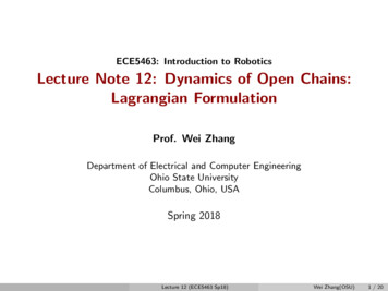
General Rigid Body Configuration683.2. Rotations and Angular Velocitiesx̂bẑbŷbẑspŷsx̂sFigure 3.6: Mathematical description of position and orientation.of rotations is provided by the exponential coordinates, which General rigid R SO(3)definean axisof rotation and theincludesangle rotatedbothabout thatWe leaveother popular representationsorientations (the three-parameter Euler anand the positionp R3 of theofrigidbody.gles and the roll–pitch–yaw angles, the Cayley–Rodrigues parameters,and the unit quaternions, which use four variables subject to one constraint)to Appendix B. Rigid body configurationcan be represented by the pair (R, p)We then examine the six-parameter exponential coordinates for the configuration of a rigid body that arise from integrating a six-dimensional twist con-sisting of the body’s angular and linear velocities. This representation follows Definition (SpecialEuclidean Group):from the Chasles–Mozzi theorem which states that every rigid-body displacement can be obtained by a finite rotation and translation about a fixed screwaxis.3SE(3) {(R,: R of SO(3),p RRather} thanSO(3) R3We concludewith ap)discussionforces and moments.treatthese as separate three-dimensional quantities, we merge the moment and forcevectors into a six-dimensional wrench. The twist and wrench, and rules formanipulating them, form the basis for the kinematic and dynamic analyses insubsequent chapters.3.2General Rigid Body MotionRotations andLectureAngularVelocities4 (ECE5463Sp18)Wei Zhang(OSU)3 / 36
Special Euclidean Group683.2. Rotations and Angular Velocitiesx̂bẑbŷbẑspŷsx̂sFigure 3.6: Mathematical description of position and orientation. Let (R, p) SE(3), where p is the coordinate of the origin of {b} in frameof rotations ofis providedby the exponentialcoordinates,{s} and R is representationthe orientation{b} relativeto {s}.Let whichqs , qb be thedefine an axis of rotation and the angle rotated about that axis. We leaveotherof orientations(the three-parameterEuler ancoordinates ofa popularpointrepresentationsq relativeto frames{s} and {b},respectively. Thengles and the roll–pitch–yaw angles, the Cayley–Rodrigues parameters,and the unit quaternions, which use four variables subject to one constraint)to Appendix B.s exponentialb coordinates for the configWe then examine the six-parameteruration of a rigid body that arise from integrating a six-dimensional twist consisting of the body’s angular and linear velocities. This representation followsfrom the Chasles–Mozzi theorem which states that every rigid-body displacement can be obtained by a finite rotation and translation about a fixed screwaxis.We conclude with a discussion of forces and moments. Rather than treatthese as separate three-dimensional quantities, we merge the moment and forcevectors into a six-dimensional wrench. The twist and wrench, and rules formanipulating them, form the basis for the kinematic and dynamic analyses insubsequent chapters.q Rq p3.2General Rigid Body MotionRotations andLectureAngularVelocities4 (ECE5463Sp18)Wei Zhang(OSU)4 / 36
Outline Representation of General Rigid Body Motion Homogeneous Transformation Matrix Twist and se(3) Twist Representation of Rigid Motion Screw Motion and Exponential CoordinateHomogeneous RepresentationLecture 4 (ECE5463 Sp18)Wei Zhang(OSU)5 / 36
Homogeneous Representation For any point x R , its homogeneous coordinate is x̃ 3 x1 0 0 Similar, homogeneous coordinate for the origin is õ 0 1 Homogeneous coordinate for a vector v is: Some rules of syntax for homogeneous coordinates:Homogeneous RepresentationLecture 4 (ECE5463 Sp18)Wei Zhang(OSU)6 / 36
Homogeneous Transformation Matrix Associate each (R, p) SE(3) with a 4 4 matrix:T R0p1 with T 1 RT0 RT p1 T defined above is called a homogeneous transformation matrix. Any rigidbody configuration (R, p) SE(3) corresponds to a homogeneoustransformation matrix T . Equivalently, SE(3) can be defined as the set of all homogeneoustransformation matrices. Slight abuse of notation: T (R, p) SE(3) and T x Rx p for x R3Homogeneous RepresentationLecture 4 (ECE5463 Sp18)Wei Zhang(OSU)7 / 36
Uses of Transformation Matrices Representation of rigid body configuration (orientation and position) Change of reference frame in which a vector or a frame is representedHomogeneous RepresentationLecture 4 (ECE5463 Sp18)Wei Zhang(OSU)8 / 36
Uses of Transformation Matrices Rigid body motion operator that displaces a vectorHomogeneous RepresentationLecture 4 (ECE5463 Sp18)Wei Zhang(OSU)9 / 36
Uses of Transformation Matrices Rigid body motion operator that displaces a frameHomogeneous RepresentationLecture 4 (ECE5463 Sp18)Wei Zhang(OSU)10 / 36
Example of Homogeneous Transformation MatrixIn terms of the coordinates of a fixed space frame {s}, frame {a} has its x̂a -axis pointing in the direction(0, 0, 1) and its ŷa -axis pointing ( 1, 0, 0), and frame {b} has its x̂b -axis pointing (1, 0, 0) and its ŷb -axispointing (0, 0, 1). The origin of {a} is at (3, 0, 0) in {s} and the origin of {b} is at (0, 2, 0) is {s}.Homogeneous RepresentationLecture 4 (ECE5463 Sp18)Wei Zhang(OSU)11 / 36
(j) Calculate the matrix exponential corresponding to the exponential coordinates of rigid-body motion Sθ (0, 1, 2, 3, 0, 0). Draw the correspondingframe relative to {s}, as well as the screw axis S.Example of Homogeneous Transformation MatrixFixed frame {a}; end effector frame {b}, the cameraframe {c}, and the workpiece frame {d}. Supposekpc pb k d1{a} ŷax̂a1Figure 3.23: Four reference frames defined in a robot’s workspace.Exercise 3.17 Four reference frames are shown in the robot workspace ofFigure 3.23: the fixed frame {a}, the end-effector frame effector {b}, the cameraframe {c}, and the workpiece frame {d}.(a) Find Tad and Tcd in terms of the dimensions given in the figure.(b) Find Tab given that 1 0 0 4 0 1 0 0 Tbc 0 0 1 0 .0 0 0 1May 2017 preprint of Modern Robotics, Lynch and Park, Cambridge U. Press, 2017. http://modernrobotics.orgHomogeneous RepresentationLecture 4 (ECE5463 Sp18)Wei Zhang(OSU)12 / 36
Outline Representation of General Rigid Body Motion Homogeneous Transformation Matrix Twist and se(3) Twist Representation of Rigid Motion Screw Motion and Exponential CoordinateTwist & se(3)Lecture 4 (ECE5463 Sp18)Wei Zhang(OSU)13 / 36
Towards Exponential Coordinate Recall: rotation matrix R SO(3) can be represented in exponentialcoordinate ω̂θ- q(θ) Rot(ω̂, θ)q0 viewed as a solution to q̇(t) [ω̂]q(t) with q(0) q0 att θ.- The above relation requires that the rotation axis passes through the origin. We can find exponential coordinate for T SE(3) using a similar approach(i.e. via differential equation) We first need to introduce some important concepts.Twist & se(3)Lecture 4 (ECE5463 Sp18)Wei Zhang(OSU)14 / 36
Differential Equation for Rigid Body Motionω Rotation about axis that may notvpass through the originp(t)p(t)pqp(a)(b)Figure 2.5: (a) A revolute joint and (b) a prismatic joint. TranslationThe solution of the differential equation is given bybTwist & se(3)bp̄(t) eξt p̄(0),b definewhere eξt is the matrix exponential of the 4 4 matrix ξt,usual) byb 3b 2bb (ξt) (ξt) · · ·eξt I ξt2!3!The scalar t is the total amount of rotation (since we are rotatingb is a mapping from the initial location of aunit velocity). exp(ξt)to its location after rotating t radians.In a similar manner, we can represent the transformation due to tlational motion as the exponential of a 4 4 matrix. The velocityLecture 4 (ECE5463 Sp18)Wei Zhang(OSU)15 / 36
Differential Equation for Rigid Body Motion Consider the following differential equation in homogeneous coordinatesṗ(t) ω p(t) v ṗ(t)0 [ω] v0 0 p(t)1 (1) The variable v contains all the constant terms (e.g. ω q in the rotationexample); thus, it may NOT be equal to the linear velocity of the origin ofthe rigid body. Solution to (1) is p(t)1 exp [ω] v0 0 p(0)t1 Motion of this form is characterized by (ω, v) which is called spatial velocityor Twist.Twist & se(3)Lecture 4 (ECE5463 Sp18)Wei Zhang(OSU)16 / 36
Twist Angular velocity and “linear” velocity can be combined to form the SpatialVelocity or TwistV ωv R6 Each twist V corresponds to a motion equation (1). For each twist V (ω, v), let [V] be its matrix representation[V] [ω] v0 0 With these notations, solution to (1) is given by Twist & se(3)p(t)1 e[V]t Lecture 4 (ECE5463 Sp18)p01 Wei Zhang(OSU)17 / 36
se(3) Similar to so(3), we can define se(3):se(3) {([ω], v) : [ω] so(3), v R3 } se(3) contains all matrix representation of twists or equivalently all twists. In some references, [V] is called a twist. We follow the textbook notation tocall the spatial velocity V (ω, v) a twist. Sometimes, we may abuse notation by writing V se(3).Twist & se(3)Lecture 4 (ECE5463 Sp18)Wei Zhang(OSU)18 / 36
Example of Twist 10 V 0 , 1 can have multiple different physical interpretations00Twist & se(3)Lecture 4 (ECE5463 Sp18)Wei Zhang(OSU)19 / 36
Outline Representation of General Rigid Body Motion Homogeneous Transformation Matrix Twist and se(3) Twist Representation of Rigid Motion Screw Motion and Exponential CoordinateTwist and Rigid MotionLecture 4 (ECE5463 Sp18)Wei Zhang(OSU)20 / 36
Exponential Map of se(3): From Twist to Rigid MotionTheorem 1.For any V (ω, v) and θ R, we have e[V]θ SE(3) I vθ Case 1 (ω 0): e[V]θ 0 1 Case 2 (ω 6 0): without loss of generality assume kωk 1. Thene[V]θ e[ω]θ0Twist and Rigid MotionG(θ)v1 , with G(θ) Iθ (1 cos(θ))[ω] (θ sin(θ))[ω]2Lecture 4 (ECE5463 Sp18)Wei Zhang(OSU)(2)21 / 36
Log of SE(3): from Rigid-Body Motion to TwistTheorem 2.Given any T (R, p) SE(3), one can always find twist V (ω, v) and a scalar θ suchthat R pe[V]θ T 0 1Matrix Logarithm Algorithm: If R I, then set ω 0, v p/kpk, and θ kpk. Otherwise, use matrix logarithm on SO(3) to determine ω and θ from R. Then v iscalculated as v G 1 (θ)p, whereG 1 (θ) Twist and Rigid Motion11I [ω] θ2 11θ cosθ22Lecture 4 (ECE5463 Sp18) [ω]2Wei Zhang(OSU)22 / 36
Example of Exponential/LogTwist and Rigid MotionLecture 4 (ECE5463 Sp18)Wei Zhang(OSU)23 / 36
Quick Summary Angular and linear velocity can be combined to form a spatial velocity ortwist V (ω, v) Each twist V (ω, v) defines a motion such that any point p on the rigidbody follows a trajectory generated by the following ODE:ṗ(t) ω p(t) v Solution to this ODE (in homogeneous coordinate): p̃(t) e[V]t p̃(0). For any twist V (ω, v) and θ R, its matrix exponential e[V]θ SE(3),i.e., it corresponds to a rigid body transformation. We have an analyticalformula to compute the exponential (Theorem 1) For any T SE(3), we also have analytical formula (Theorem 2) to findV (ω, v) and θ R such at e[V]θ T .Twist and Rigid MotionLecture 4 (ECE5463 Sp18)Wei Zhang(OSU)24 / 36
Outline Representation of General Rigid Body Motion Homogeneous Transformation Matrix Twist and se(3) Twist Representation of Rigid Motion Screw Motion and Exponential CoordinateScrew Motion and Exp. CoordinateLecture 4 (ECE5463 Sp18)Wei Zhang(OSU)25 / 36
Screw Interpretation of Twist Given a twist V (ω, v), the associated motion (1) may have differentinterpretations (different rotation axes, linear velocities). We want to impose some nominal interpretable structure on the motion. Recall: an angular velocity vector ω can be viewed as ω̂ θ̇, where ω̂ is the unitrotation axis and θ̇ is the rate of rotation about that axis Similarly, a twist (spatial velocity) V can be interpreted in terms of a screwaxis S and a velocity θ̇ about the screw axisScrew Motion and Exp. CoordinateLecture 4 (ECE5463 Sp18)Wei Zhang(OSU)26 / 36
Screw Motion: DefinitionChapter 3. Rigid-Body Motions Rotating about an axis while also translating along the axis103ŝẑhŝθ̇θ̇ ŝθ̇ qx̂qŷh pitch linear speed/angular speedFigureA screwrepresenteda point q, a speedunit direction Representedby 3.19:screwaxisaxis{q,S ŝ,h} andbyrotationθ̇ ŝ, and a pitchh.- ŝ: unit vector in the direction of the rotation axisA screw axis represents the familiar motion of a screw: rotating about thethe axis. One representation of a screw axisS is the collection {q, ŝ, h}, where q R3 is any point on the axis, ŝ is a unitvector in the direction of the axis, and h is the screw pitch, which defines the- h: screwratiopitchwhichthe ratioof thevelocityalongθ̇ aboutthe screwof thelinear definesvelocity alongthe screwaxis linearto the angularvelocitythe screwvelocityaxis (Figure3.19).to the angularaboutthe screw axisUsing Figure 3.19 and geometry, we can write the twist V (ω, v) corresponding to an angular velocity θ̇ about S (represented by {q, ŝ, h}) as ωŝθ̇V .v 4 (ECE5463Screw Motion and Exp. CoordinateLectureWei Zhang(OSU) ŝθ̇Sp18) q hŝθ̇axis whilealso rotationtranslatingaxisalong- q: any pointon theaxis27 / 36
Screw Motion as Solution to ODE Consider a point p on a rigid body under a screw motion with (rotation)speed θ̇. Let p(t) be its coordinate at time t. The overall velocity isṗ(t) ŝθ̇ (p(t) q) hŝθ̇(3) Thus, any screw axis {q, ŝ, h} with rotation speed θ̇ can be represented by aparticular twist (ω, v) with ω ŝθ̇ and v ŝθ̇ q hŝθ̇.Screw Motion and Exp. CoordinateLecture 4 (ECE5463 Sp18)Wei Zhang(OSU)28 / 36
From Twist to Screw Axis The converse is true as well: given any twist V (ω, v) one can always find{q, ŝ, h} and θ̇ such that the corresponding screw motion (eq. (3)) coincideswith the motion generated by the twist (eq. (1)).- If ω 0, then it is a pure translation (h )- If ω 6 0:Screw Motion and Exp. CoordinateLecture 4 (ECE5463 Sp18)Wei Zhang(OSU)29 / 36
Examples Screw Axis and Twist What is the twist that corresponds torotating about ẑb ?ωzAxθByql1Figure 2.9: Rigid body motion generated by rotation about a fi What is the screw axis for twist V (0, 2, 2, 4, 0, 0)?q (0, l1 , 0). The corresponding twist is l 1 0 ω q 00 .ξ ω01Screw Motion and Exp. CoordinateThe exponential of this twist is given by cos θ sin θ 0l1 sin ωb θ sin θ Wei cosLecture4e(ECE5463Zhang(OSU)/ 36θ 0 l30(1 b(ISp18) eωb θ )(ω v)
Implicit Definition of Screw Axis for a Given a Twist For any twist V (ω, v), we can always view it as a ”screw velocity” thatconsists an screw axis S and the velocity θ̇ about the screw axis. Instead of using {q, ŝ, h} to represent S, we adopt a more convenientrepresentation defined below: Screw axis (corresponding to a twist): Given any twist V (ω, v), itsscrew axis is defined as- If ω 6 0, then S : V/kωk (ω/kωk, v/kωk).- If ω 0, then S : V/kvk (0, v/kvk)Screw Motion and Exp. CoordinateLecture 4 (ECE5463 Sp18)Wei Zhang(OSU)31 / 36
Unit Screw Axis (unit) screw axis S can be represented byS ωv R6where either (i)kωk 1 or (ii) ω 0 and kvk 1 We have used (ω, v) to represent both screw axis (where kωk or kvk 1must be unity) and a twist (where there are no constrains on ω and v) S (w, v) is called a screw axis, but we typically do not bother to explicitlyfind the corresponding {q, ŝ, h}. We can find them whenever needed.Screw Motion and Exp. CoordinateLecture 4 (ECE5463 Sp18)Wei Zhang(OSU)32 / 36
Exponential Coordinates of Rigid Transformation Screw axis S (ω, v) is just a normalized twist; its matrix representation is[S] [ω] v0 0 se(3) Therefore, a point started at p(0) at time zero, travel along screw axis S atunit speed for time t will end up at p(t) e[S]t p(0) Given S we can use Theorem 1 to compute e[S]t SE(3); Given T SE(3), we can use Theorem 2 to find S (ω, v) and θ such thate[S]θ T . We call Sθ the Exponential Coordinate of the homogeneoustransformation T SE(3)Screw Motion and Exp. CoordinateLecture 4 (ECE5463 Sp18)Wei Zhang(OSU)33 / 36
Show that the twist of {a} in space-frame coordinates is the same as theof {b} in space-frame coordinates.Example of Exponential ŷ01x̂1(a) A first screw {1}(b) A second screw motion.Figure 3.32: A cube undergoing two different screw motions.Exercise 3.30 A cube undergoes two different screw motions from framto frame {2} as shown in Figure 3.32. In both cases, (a) and (b), theconfiguration of the cube is 1 0 0 0 0 1 0 1 T01 0 0 1 0 .Screw Motion and Exp. CoordinateLecture 4 (ECE5463 Sp18)Wei Zhang(OSU)34 / 36
More DiscussionsScrew Motion and Exp. CoordinateLecture 4 (ECE5463 Sp18)Wei Zhang(OSU)35 / 36
More DiscussionsScrew Motion and Exp. CoordinateLecture 4 (ECE5463 Sp18)Wei Zhang(OSU)36 / 36
3.2 Rotations and Angular Velocities 3.2.1 Rotation Matrices We argued earlier that, of the nine entries in the rotation matrix R, only three can be chosen independently. We begin by expressing a set of six explicit con-straints on the entries of R. Recall that the three columns of R correspond to