WIXLIB

ECE5463: Introduction to RoboticsLecture Note 12: Dynamics of Open Chains:Lagrangian FormulationProf. Wei ZhangDepartment of Electrical and Computer EngineeringOhio State UniversityColumbus, Ohio, USASpring 2018Lecture 12 (ECE5463 Sp18)Wei Zhang(OSU)1 / 20

Outline Introduction Euler-Lagrange Equations Lagrangian Formulation of Open-Chain DynamicsOutlineLecture 12 (ECE5463 Sp18)Wei Zhang(OSU)2 / 20

From Single Rigid Body to Open Chains Recall Newton-Euler Equation for a single rigid body:TFb Gb V̇b [adVb ] (Gb Vb ) Open chains consist of multiple rigid links connected through joints Dynamics of adjacent links are coupled. We are concerned with modeling multi-body dynamics subject to constraints.IntroductionLecture 12 (ECE5463 Sp18)Wei Zhang(OSU)3 / 20

Preview of Open-Chain Dynamics Equations of Motion are a set of 2nd-order differential equations:τ M (θ)θ̈ h(θ, θ̇)- θ Rn : vector of joint variables; τ Rn : vector of joint forces/torques- M (θ) Rn n : mass matrix- h(θ, θ̇) Rn : forces that lump together centripetal, Coriolis, gravity, and frictionterms that depend on θ and θ̇ Forward dynamics: Determine acceleration θ̈ given the state (θ, θ̇) and thejoint forces/torques:θ̈ M 1 (θ)(τ h(θ, θ̇)) Inverse dynamics: Finding torques/forces given state (θ, θ̇) and desiredacceleration θ̈τ M (θ)θ̈ h(θ, θ̇)IntroductionLecture 12 (ECE5463 Sp18)Wei Zhang(OSU)4 / 20

Lagrangian vs. Newton-Euler Methods There are typically two ways to derive the equation of motion for anopen-chain robot: Lagrangian method and Newton-Euler methodNewton-Euler FormulationLagrangian Formulation- Energy-based method- Balance of forces/torques- Dynamic equations in closedform- Dynamic equations innumeric/recursive form- Often used for study of dynamicproperties and analysis ofcontrol methods- Often used for numericalsolution of forward/inversedynamicsIntroductionLecture 12 (ECE5463 Sp18)Wei Zhang(OSU)5 / 20

Outline Introduction Euler-Lagrange Equations Lagrangian Formulation of Open-Chain DynamicsEuler-Lagrange EquationsLecture 12 (ECE5463 Sp18)Wei Zhang(OSU)6 / 20

Generalized Coordinates and Forces Consider k particles. Let fi be the force acting on the ith particle, m̄i be itsmass, pi be its position. Newton’s law: fi m̄i p̈i ,i 1, . . . k Now consider the case in which some particles are rigidly connected,imposing constraints on their positionsαj (p1 , . . . , pk ) 0,j 1, . . . , nc k particles in R3 under nc constraints 3k nc degree of freedom Dynamics of this constrained k-particle system can be represented byn , 3k nc independent variables qi ’s, called the generalized coordinates((αj (p1 , . . . , pk ) 0pi γi (q1 , . . . , qn ) j 1, . . . , nci 1, . . . , kEuler-Lagrange EquationsLecture 12 (ECE5463 Sp18)Wei Zhang(OSU)7 / 20

Generalized Coordinates and Forces To describe equation of motion in terms of generalized coordinates, we alsoneed to express external forces applied to the system in terms componentsalong generalized coordinates. These “forces” are called generalized forces. Generalized force fi and coordinate rate q̇i are dual to each other in the sensethat f T q̇ corresponds to power The equation of motion of the k-particle system can thus be described interms of 3k nc independent variables instead of the 3k position variablessubject to nc constraints. This idea of handling constraints can be extended to interconnected rigidbodies (open chains).Euler-Lagrange EquationsLecture 12 (ECE5463 Sp18)Wei Zhang(OSU)8 / 20

Euler-Lagrange Equation Now let q Rn be the generalized coordinates and f Rn be thegeneralized forces of some constrained dynamical system. Lagrangian function: L(q, q̇) K(q, q̇) P(q)- K(q, q̇): kinetic energy of system- P(q): potential energy Euler-Lagrange Equations:f Euler-Lagrange Equationsd L L dt q̇ qLecture 12 (ECE5463 Sp18)(1)Wei Zhang(OSU)9 / 20

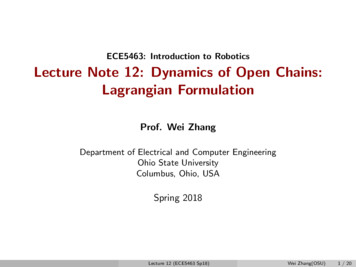
Example: Spherical PendulumlθφmgFigure 4.1: Idealized spherical pendulum. The configtem is described by the angles θ and φ. Lwhere L q̇ , q , and Υ are to be formally regarded as rwe often write them as column vectors for notationproof of Theorem 4.1 can be found in most books ochanical systems (e.g., [99]).Lagrange’s equations are an elegant formulationa mechanical system. They reduce the number of edescribe the motion of the system from n, the numbesystem, to m, the number of generalized coordinates.are no constraints,then we can choose q to be the comPmi kṙi2 k, and equation (4.5) then reduces toT 21fact, rearranging equation (4.5) asEuler-Lagrange EquationsLecture 12 (ECE5463 Sp18) Ld L Υdt q̇ qWei Zhang(OSU)10 / 20

Example: Spherical Pendulum (Continued)Euler-Lagrange EquationsLecture 12 (ECE5463 Sp18)Wei Zhang(OSU)11 / 20

Outline Introduction Euler-Lagrange Equations Lagrangian Formulation of Open-Chain DynamicsLagrangian FormulationLecture 12 (ECE5463 Sp18)Wei Zhang(OSU)12 / 20

Lagrangian Formulation of Open Chains For open chains with n joints, it is convenient and always possible to choosethe joint angles θ (θ1 , . . . , θn ) and the joint torques τ (τ1 , . . . , τn ) as thegeneralized coordinates and generalized forces, respectively.- If joint i is revolute: θi joint angle and τi is joint torque- If joint i is prismatic: θi joint position and τi is joint force Lagrangian function: L(θ, θ̇) K(θ, θ̇) P(θ, θ̇) Dynamic Equations:τi d L L dt θ̇i θi To obtain the Lagrangian dynamics, we need to derive the kinetic andpotential energies of the robot in terms of joint angles θ and torques τ .Lagrangian FormulationLecture 12 (ECE5463 Sp18)Wei Zhang(OSU)13 / 20

Some NotationsFor each link i 1, . . . , n, Frame {i} is attached to the center of mass of link i.All the following quantities are expressed in frame {i} Vi : Twist of link {i} m̄i : mass; Gi Ii0Ii : rotational inertia matrix;0m̄i I : Spatial inertia matrix Kinetic energy of link i: Ki 21 ViT Gi Vi Jb(i) R6 i : body Jacobian of link ih(i)(i)Jb Jb,1h(i)where Jb,j AdLagrangian Formulationie [Bi ]θi ···e [Bj 1 ]θj 1.(i)Jb,ii(i)Bj , j i and Jb,i BiLecture 12 (ECE5463 Sp18)Wei Zhang(OSU)14 / 20

Kinetic and Potential Energies of Open Chains(i) Jib [Jb0] R6 n Total Kinetic Energy:K(θ, θ̇) 1 Xn1 Xn1TViT Gi Vi θ̇TJib(θ)Gi Jib (θ) θ̇ , θ̇T M (θ)θ̇i 1i 1222 Potential Energy:P(θ) Xni 1m̄i ghi (θ)- hi (θ): height of CoM of link iLagrangian FormulationLecture 12 (ECE5463 Sp18)Wei Zhang(OSU)15 / 20

Lagrangian Dynamic Equations of Open Chains Lagrangian: L(θ, θ̇) K(θ, θ̇) P(θ) τi d Ldt θ̇i τi L θinXi j Mij (θ)θ̈j n XnXΓijk (θ)θ̇j θ̇k j 1 k 1 P, θii 1, . . . , n Γijk (θ) is called the Christoffel symbols of the first kind 1 Mij Mik Mjk Γijk (θ) 2 θk θj θiLagrangian FormulationLecture 12 (ECE5463 Sp18)Wei Zhang(OSU)16 / 20

Lagrangian Dynamic Equations of Open Chains Dynamic equation in vectorform:To compute themanipulator inertia matrix, we first compute the bodyJacobians corresponding to each link frame. A detailed, but straightforward, calculation yields r1 c2 0 0 0 0 0 τ J M (θ)θ̈ J C(θ,θ̇)θ̇ g(θ) J J1- Cij (θ, θ̇) ,Pnk 13θ300000000002 lL3L1L4bsl3 (0)2 c2 r2 c23000 s23c23The inertia matrix M11M (θ) M21M31for the system is given byΓ112 (Iy2 Iz2 m2 r12 )c2 s2 (Iy3 Iz3 )c23 s23 m3 (l1 c2 r2 c23 )(l1 s2 r2 s23 )M12 M13M22 M23 J1T M1 J1 J2T M2 J2 J3T M3 J3 . Γ113 (Iy3 Iz3 )c23 s23 m3 r2 s23 (l1 c2 r2 c23 )M32 M33Γ121 (Iy2 Iz2 m2 r12 )c2 s2 (Iy3 Iz3 )c23 s23 m3 (l1 c2 r2 c23 )(l1 s2 r2 s23 )The components of M are given byθ4yΓ211 (Iz2 Iy2 m2 r12 )c2 s2 (Iz3 Iy3 )c23 s23M21 0Γ223 l1 m3 r2 s3M22 Ix2 Ix3 m3 l12 m2 r12 m3 r22 2m3 l1 r2 c3M31 0M32 Ix3 m3 r22 m3 l1 r2 c3l2Γ131 (Iy3 Iz3 )c23 s23 m3 r2 s23 (l1 c2 r2 c23 )M12 0M13 0M23 Ix3 m3 r22 m3 l1 r2 c3l0l100000 m2 r12 c22 m3 (l1 c2 r2 c23 )2L2z000 r10 1 s20c20 00l1 s 30 r2 l1 c3 r2 1 1 .0000 by:bsl2 (0)M11 Iy2 s22 Iy3 s223 Iz1 Iz2 c22 Iz3 c223θ1S00001Γijk θ̇k is calledtheCoriolis matrix J J θ2xbsl1 (0)M33 Ix3 m3 r22 . m3 (l1 c2 r2 c23 )(l1 s2 r2 s23 )Γ232 l1 m3 r2 s3Γ233 l1 m3 r2 s3Γ311 (Iz3 Iy3 )c23 s23 m3 r2 s23 (l1 c2 r2 c23 )Γ322 l1 m3 r2 s3Note that several of the moments of inertia of the differentFinally,links dowenotcompute the effect of gravitational forces on the manipuappear in this expression. This is because the limited degreesof freedomderivative giveslator. Theseforces are written asof the manipulatordo not allow arbitrary rotations of each joint aroundFigure 4.6: SCARA manipulator in its reference configuration.0 Veach V axis. ,N (θ, θ̇) forcesaremcomputed (m2andgr1 centrifugal m3 gl1 ) cosθ2 θ3 )) from. theN (θ, θ̇) The Coriolis θ3 r2 cos(θ2directly θ matrix via the formulainertiawhere m3 gr2 cos(θ2 θ3 ))n2222where V : R R is the potential energy of the manipulator. For theα Iz1 r1 m1 l1 m2 l1 m3 l1 m4nn XX1 Mik three-link Mkj MijΓijk θ̇k Cij (θ, θ̇) θ̇k .manipulator under consideration here, the potential energy isβ Iz2 Iz3 Iz4 l22 m3 l22 m4 m2 r222 θk θj θi bygivenk 1k 1(4.25)γ l1 l2 m3 l1 l2 m4 l1 m2 r2This completes the derivation of the dynamics.V (θ) m1 gh1 (θ) m2 gh2 (θ) m3 gh3 (θ),A very messy calculationthat the nonzerovalues of Γijk are givenLectureshows12 (ECE5463Sp18)Wei Zhang(OSU)17 / 20δ LagrangianIz3 Iz4 . Formulation