Transcription
Exercise 1: Intro to COMSOL (revised)Transport in Biological SystemsFall 2015OverviewIn this course, we will consider transport phenomena in biological systems. Generally speaking, biologicalsystems of interest have interesting geometries and we are interested in things happening in time and space.This means that analytical solutions can be challenging to find. Therefore, a modeling and simulationapproach is often useful. Towards this, we will employ COMSOL in this course. It takes a little bit to getup to speed but it’s a very powerful tool.You will work on this in class (AC318) on September 3rd, the first day of class. Alisha will not be present,but you should all work as a group on this. Please try to complete the first 3 training items beforeclass.Training1. Install COMSOL on your computer if you haven’t (http://wikis.olin.edu/it/doku.php?id comsol).2. Read: oductionToCOMSOLMultiphysics.pdf3. Watch: tiphysics-a-tutorial-video/4. Attend the COMSOL training from 9:30-12:30 on September 17th. (Note: I know a few of you haveclass before this one. Please come as soon as you can. If it is acceptable for your other class to leaveearly on that day, it would be great, but I also understand if you can’t.)Exercises1. Make a smiley face (Figure 1, which I cannot get LaTex to put here and seems to be at the end!).Hint: think about using ellipses and intersections, not lines for the smile.1
2. Make a hollow sphere with holes in it (Figure 2). Don’t worry about dimensions, just the generalconcept.Figure 2: A hollow sphere with holes.3. Do the 2 exercises attached at the end of this document. (credit: COMSOL)Objectives and DeliverablesThe objective of this course is for you to apply concepts and skills in modeling and simulation to problemsin biological transport. The objectives of this particular exercise are to gain practice using COMSOL.Complete the exercises and provide figures showing the final results for the exercises you have completed.It doesn’t have to be anything pretty. Your results are due by September 21st.2
Solved with COMSOL Multiphysics 5.1Cooling and Solidification of MetalIntroductionThis example is a model of a continuous casting process. Liquid metal is poured intoa mold of uniform cross section. The outside of the mold is cooled and the metalsolidifies as it flows through the mold. When the metal leaves the mold, it is completelysolidified on the outside but still liquid inside. The metal then continues to cool andeventually solidify completely, at which point it can be cut into sections. This tutorialsimplifies the problem somewhat by not computing the flow field of the liquid metaland assuming there is no volume change at solidification. It is also assumed that thevelocity of the metal is constant and uniform throughout the modeling domain. Thephase transition from molten to solid state is modeled via the apparent heat capacityformulation. Issues of convergence and mesh refinement are addressed for this highlynonlinear model.The Continuous Casting application is similar to this one, except that the velocity iscomputed from the Laminar Flow interface instead of being considered constant anduniform. For a detailed description of the application, see Continuous Casting.Molten metalTundishNozzleCooled moldSpray coolingSawModeling regionSolid metal billetFigure 1: A continuous casting process. The section where the metal is solidifying is beingmodeled.1 COOLING AND SOLIDIFICATION OF METAL
Solved with COMSOL Multiphysics 5.1Model OverviewThe model simplifies the 3D geometry of the continuous casting to a 2D axisymmetricmodel composed of two rectangular regions: one representing the strand within themold, and one the spray cooled region outside of the mold, prior to the saw cutoff. Inthe second section, there is also significant cooling via radiation to the ambient. In thisregion it is assumed that the molten metal is in a hydrostatic state, that the only motionin the fluid is due to the bulk downward motion of the strand. This simplificationallows the assumption of bulk motion throughout the domain.Since this is a continuous process, the system can be modeled at steady state. The heattransport is described by the equation: ( – k T ) – ρC p u Twhere k and Cp denote thermal conductivity and specific heat, respectively. Thevelocity, u, is the fixed casting speed of the metal in both liquid and solid states.As the metal cools down in the mold, it solidifies. During the phase transition, asignificant amount of latent heat is released. The total amount of heat released per unitmass of alloy during the transition is given by the change in enthalpy, ΔH. In addition,the specific heat capacity, Cp, also changes considerably during the transition. Thedifference in specific heat before and after transition can be approximated byΔHΔC p --------TAs opposed to pure metals, an alloy generally undergoes a broad temperaturetransition zone, over several Kelvin, in which a mixture of both solid and moltenmaterial co-exist in a “mushy” zone. To account for the latent heat related to the phasetransition, the Apparent Heat capacity method is used through the Heat Transfer withPhase Change domain condition. The objective of the analysis is to make ΔT, thehalf-width of the transition interval small, such that the solidification front location iswell defined.Table 1 reviews the material properties in this tutorial.TABLE 1: MATERIAL PROPERTIESPROPERTYDensity2 COOLING AND SOLIDIFICATION OF METALSYMBOL3ρ (kg/m )MELTSOLID85008500
Solved with COMSOL Multiphysics 5.1PROPERTYSYMBOLMELTSOLIDHeat capacity at constant pressureCp (J/(kg K))531380Thermal conductivityk (W/(m K))150300The melting temperature, Tm, and enthalpy, ΔH, are 1356 K and 205 kJ/kg,respectively.This example is a highly nonlinear problem and benefits from taking an iterativeapproach to finding the solution. The location of the transition between the moltenand solid state is a strong function of the casting velocity, the cooling rate in the mold,and the cooling rate in the spray cooled region. A fine mesh is needed across thesolidification front to resolve the change in material properties. However, it is notknown where this front will be.By starting with a gradual transition between liquid and solid, it is possible to find asolution even on a relatively coarse mesh. This solution can be used as the startingpoint for the next step in the solution procedure, which uses a sharper transition fromliquid to solid. This is done using the continuation method. Given a monotonic list ofvalues to solve for, the continuation method uses the solution to the last case as thestarting condition for the next. Once a solution is found for the smallest desired ΔT,the adaptive mesh refinement algorithm is used to refine the mesh to put moreelements around the transition region. This finer mesh is then used to find a solutionwith an even sharper transition. This can be repeated as needed to get better and betterresolution of the location of the solidification front.In this example, the parameter ΔT is first ramped down from 300 K to 75 K, then theadaptive mesh refinement is used such that a finer mesh is used around thesolidification front. The resultant solution and mesh are then used as starting pointsfor a second study, where the parameter ΔT is further ramped down from 50 K to25 K. The double-dogleg solver is used to find the solution to this highly nonlinearproblem. Although it takes more time, this solver converges better in cases whenmaterial properties vary strongly with respect to the solution.Results and DiscussionThe solidification front computed with the coarsest mesh, and for ΔT 75 K, is shownin Figure 2. A wide transition between the molten and solid state is observed. Theadaptive mesh refinement algorithm then refines the mesh along the solidificationfront because this is the region where the results are strongly dependent upon meshsize. This solution, and refined mesh, is used as the starting point for the next solution,3 COOLING AND SOLIDIFICATION OF METAL
Solved with COMSOL Multiphysics 5.1which ramps the ΔT parameter down to 25 K. These results are shown in Figure 3.The point of complete solidification moves slightly as the transition zone is madesmaller. As the transition zone becomes smaller, a finer mesh is needed, otherwise themodel might not converge. If it is desired to get an even better resolution of thesolidification front, the solution procedure used here should be repeated to get an evenfiner mesh, and further ramp down the ΔT parameter.The liquid phase fraction is plotted along the r-direction at the line at the bottom ofthe mold in Figure 4, and Figure 5 shows the liquid fraction along the centerline ofthe strand. For smaller values of ΔT, the transition becomes sharper, and the modelgives confidence that the metal is completely solidified before the strand is cut.Figure 2: The fraction of liquid phase for ΔT 75 K shows a gradual transition betweenthe liquid and solid phase.4 COOLING AND SOLIDIFICATION OF METAL
Solved with COMSOL Multiphysics 5.1Figure 3: The fraction of liquid phase for ΔT 25 K shows a sharp transition between theliquid and solid phase.5 COOLING AND SOLIDIFICATION OF METAL
Solved with COMSOL Multiphysics 5.1Figure 4: The fraction of liquid phase through the radius for all values of ΔT. For smallervalues of ΔT, the transition is sharper.6 COOLING AND SOLIDIFICATION OF METAL
Solved with COMSOL Multiphysics 5.1Figure 5: The fraction of liquid phase along the centerline for all values of ΔT. For smallervalues of ΔT, the transition is sharper.Application Library path: Heat Transfer Module/Thermal Processing/cooling solidification metalModeling InstructionsFrom the File menu, choose New.NEW1 In the New window, click Model Wizard.MODEL WIZARD1 In the Model Wizard window, click 2D Axisymmetric.2 In the Select physics tree, select Heat Transfer Heat Transfer in Fluids (ht).3 Click Add.4 Click Study.7 COOLING AND SOLIDIFICATION OF METAL
Solved with COMSOL Multiphysics 5.15 In the Select study tree, select Preset Studies Stationary.6 Click Done.GLOBAL DEFINITIONSFirst, set up parameters and variables used in the continuous casting process modelanalysis.Parameters1 On the Home toolbar, click Parameters.2 In the Settings window for Parameters, locate the Parameters section.3 Click Load from File.4 Browse to the application’s Application Library folder and double-click the filecooling solidification metal parameters.txt.GEOMETRY 1Create two rectangles representing the strand within the mold, and spray cooledregion outside of the mold.Rectangle 1 (r1)1 On the Geometry toolbar, click Primitives and choose Rectangle.2 In the Settings window for Rectangle, locate the Size section.3 In the Width text field, type 0.1.4 In the Height text field, type 0.6.Rectangle 2 (r2)1 On the Geometry toolbar, click Primitives and choose Rectangle.2 In the Settings window for Rectangle, locate the Size section.3 In the Width text field, type 0.1.4 In the Height text field, type 0.2.5 Locate the Position section. In the z text field, type 0.6.6 Click the Build All Objects button.8 COOLING AND SOLIDIFICATION OF METAL
Solved with COMSOL Multiphysics 5.17 Click the Zoom Extents button on the Graphics toolbar.MATERIALSMaterial 1 (mat1)1 In the Model Builder window, under Component 1 (comp1) right-click Materials andchoose Blank Material.2 In the Settings window for Material, type Solid Metal Alloy in the Label text field.3 Locate the Material Contents section. In the table, enter the following settings:PropertyNameValueUnitProperty groupThermal asicHeat capacity at constant pressureCpCp sJ/(kg·K)BasicRatio of specific heatsgamma11BasicMaterial 2 (mat2)1 In the Model Builder window, right-click Materials and choose Blank Material.2 In the Settings window for Material, type Liquid Metal Alloy in the Label textfield.3 Select Domains 1 and 2 only.9 COOLING AND SOLIDIFICATION OF METAL
Solved with COMSOL Multiphysics 5.14 Locate the Material Contents section. In the table, enter the following settings:PropertyNameValueUnitProperty groupThermal asicHeat capacity at constant pressureCpCp lJ/(kg·K)BasicRatio of specific heatsgamma11BasicSet up the physics.H E A T TR A N S F E R I N F L U I D S ( H T )Initial Values 11 In the Model Builder window, under Component 1 (comp1) Heat Transfer in Fluids (ht)click Initial Values 1.2 In the Settings window for Initial Values, locate the Initial Values section.3 In the T text field, type T in.Heat Transfer with Phase Change 11 On the Physics toolbar, click Domains and choose Heat Transfer with Phase Change.2 Select Domains 1 and 2 only.3 In the Settings window for Heat Transfer with Phase Change, locate the Model Inputssection.4 Specify the u vector as0r-v castz5 Locate the Phase Change section. In the Tpc,1 2 text field, type T m.6 In the ΔT1 2 text field, type dT.7 In the L1 2 text field, type dH.8 Locate the Phase 1 section. From the Material, phase 1 list, choose Solid Metal Alloy(mat1).9 Locate the Phase 2 section. From the Material, phase 2 list, choose Liquid Metal Alloy(mat2).Temperature 11 On the Physics toolbar, click Boundaries and choose Temperature.10 COOLING AND SOLIDIFICATION OF METAL
Solved with COMSOL Multiphysics 5.12 Select Boundary 5 only.3 In the Settings window for Temperature, locate the Temperature section.4 In the T0 text field, type T in.Heat Flux 11 On the Physics toolbar, click Boundaries and choose Heat Flux.11 COOLING AND SOLIDIFICATION OF METAL
Solved with COMSOL Multiphysics 5.12 Select Boundary 7 only.3 In the Settings window for Heat Flux, locate the Heat Flux section.4 Click the Convective heat flux button.5 In the h text field, type h mold.6 In the Text text field, type T0.Heat Flux 21 On the Physics toolbar, click Boundaries and choose Heat Flux.12 COOLING AND SOLIDIFICATION OF METAL
Solved with COMSOL Multiphysics 5.12 Select Boundary 6 only.3 In the Settings window for Heat Flux, locate the Heat Flux section.4 Click the Convective heat flux button.5 In the h text field, type h spray.6 In the Text text field, type T0.Diffuse Surface 11 On the Physics toolbar, click Boundaries and choose Diffuse Surface.2 Select Boundary 6 only.3 In the Settings window for Diffuse Surface, locate the Surface Emissivity section.4 From the ε list, choose User defined. In the associated text field, type eps s.5 Locate the Ambient section. In the Tamb text field, type T0.Outflow 11 On the Physics toolbar, click Boundaries and choose Outflow.13 COOLING AND SOLIDIFICATION OF METAL
Solved with COMSOL Multiphysics 5.12 Select Boundary 2 only.MESH 11 In the Model Builder window, under Component 1 (comp1) click Mesh 1.2 In the Settings window for Mesh, locate the Mesh Settings section.3 From the Element size list, choose Extremely fine.STUDY 11 In the Model Builder window, click Study 1.2 In the Settings window for Study, locate the Study Settings section.3 Clear the Generate default plots check box.Step 1: StationarySet up an auxiliary continuation sweep for the dT parameter.1 In the Model Builder window, under Study 1 click Step 1: Stationary.2 In the Settings window for Stationary, click to expand the Study extensions section.3 Locate the Study Extensions section. Select the Auxiliary sweep check box.4 Click Add.14 COOLING AND SOLIDIFICATION OF METAL
Solved with COMSOL Multiphysics 5.15 In the table, enter the following settings:Parameter nameParameter value listParameter unitdT300 200 150 100 756 Select the Adaptive mesh refinement check box.Solution 11 On the Study toolbar, click Show Default Solver.2 In the Model Builder window, expand the Solution 1 node.3 In the Model Builder window, expand the Study 1 Solver Configurations Solution1 Stationary Solver 1 node, then click Adaptive Mesh Refinement.4 In the Settings window for Adaptive Mesh Refinement, locate the Mesh Refinementsection.5 From the Refinement method list, choose Mesh initialization.6 In the Model Builder window, under Study 1 Solver Configurations Solution1 Stationary Solver 1 click Fully Coupled 1.7 In the Settings window for Fully Coupled, click to expand the Method andtermination section.8 Locate the Method and Termination section. From the Nonlinear method list, chooseDouble dogleg.9 On the Study toolbar, click Compute.RESULTS2D Plot Group 11 On the Home toolbar, click Add Plot Group and choose 2D Plot Group.2 In the Settings window for 2D Plot Group, type Solid and Liquid Phases(Adaptive Mesh) in the Label text field.Solid and Liquid Phases (Adaptive Mesh)1 Right-click Results Solid and Liquid Phases (Adaptive Mesh) and choose Surface.2 In the Settings window for Surface, click Replace Expression in the upper-right cornerof the Expression section. From the menu, choose Model Component 1 Heat Transferin Fluids Phase change ht.theta1 - Phase indicator, phase 1.3 On the Solid and Liquid Phases (Adaptive Mesh) toolbar, click Plot.The reproduced figure describes the fraction of liquid phase for ΔT 75 K.15 COOLING AND SOLIDIFICATION OF METAL
Solved with COMSOL Multiphysics 5.1ADD STUDY1 On the Home toolbar, click Add Study to open the Add Study window.2 Go to the Add Study window.3 Find the Studies subsection. In the Select study tree, select Preset Studies.4 In the Select study tree, select Preset Studies Stationary.5 Click Add Study in the window toolbar.STUDY 2Step 1: Stationary1 On the Home toolbar, click Add Study to close the Add Study window.2 In the Model Builder window, click Study 2.3 In the Settings window for Study, locate the Study Settings section.4 Clear the Generate default plots check box.5 In the Model Builder window, click Step 1: Stationary.6 In the Settings window for Stationary, click to expand the Values of dependentvariables section.7 Locate the Values of Dependent Variables section. Select the Initial values of variablessolved for check box.8 From the Method list, choose Solution.9 From the Study list, choose Study 1, Stationary.10 From the Solution list, choose Adaptive Mesh Refinement 1.11 From the Parameter value (dT) list, choose 75.12 Click to expand the Mesh selection section. Locate the Study Extensions section.Select the Auxiliary sweep check box.13 Click Add.14 In the table, enter the following settings:Parameter nameParameter value listdT50 25Solution 31 On the Study toolbar, click Show Default Solver.2 In the Model Builder window, expand the Solution 3 node.16 COOLING AND SOLIDIFICATION OF METALParameter unit
Solved with COMSOL Multiphysics 5.13 In the Model Builder window, expand the Study 2 Solver Configurations Solution3 Stationary Solver 1 node, then click Fully Coupled 1.4 In the Settings window for Fully Coupled, locate the Method and Terminationsection.5 From the Nonlinear method list, choose Double dogleg.6 On the Study toolbar, click Compute.RESULTS2D Plot Group 21 On the Home toolbar, click Add Plot Group and choose 2D Plot Group.2 In the Settings window for 2D Plot Group, type Solid and Liquid Phases in theLabel text field.3 Locate the Data section. From the Data set list, choose Study 2/Solution 3.Solid and Liquid Phases1 Right-click Results Solid and Liquid Phases and choose Surface.2 In the Settings window for Surface, click Replace Expression in the upper-right cornerof the Expression section. From the menu, choose Model Component 1 Heat Transferin Fluids Phase change ht.theta1 - Phase indicator, phase 1.3 On the Solid and Liquid Phases toolbar, click Plot.This shows the fraction of liquid phase for ΔT 25 K.1D Plot Group 31 On the Home toolbar, click Add Plot Group and choose 1D Plot Group.2 In the Settings window for 1D Plot Group, type Phase Indicator at SymmetryAxis in the Label text field.Phase Indicator at Symmetry Axis1 On the Phase Indicator at Symmetry Axis toolbar, click Line Graph.2 Select Boundaries 1 and 3 only.3 In the Settings window for Line Graph, locate the y-axis data section.4 Click ht.theta1 - Phase indicator, phase 1 in the upper-right corner of the section.Locate the x-Axis Data section. From the Parameter list, choose Expression.5 In the Expression text field, type z.6 Click to expand the Legends section. Select the Show legends check box.17 COOLING AND SOLIDIFICATION OF METAL
Solved with COMSOL Multiphysics 5.17 Right-click Results Phase Indicator at Symmetry Axis Line Graph 1 and chooseDuplicate.8 In the Settings window for Line Graph, locate the Data section.9 From the Data set list, choose Study 2/Solution 3.10 On the Phase Indicator at Symmetry Axis toolbar, click Plot.Compare the resulting plot with Figure 5 showing the fraction of liquid phasethrough the centerline for all values of ΔT.Phase Indicator at Symmetry Axis 11 In the Model Builder window, right-click Phase Indicator at Symmetry Axis and chooseDuplicate.2 In the Settings window for 1D Plot Group, type Phase Indicator throughRadius in the Label text field.Phase Indicator through Radius1 In the Model Builder window, expand the Results Phase Indicator through Radiusnode, then click Line Graph 1.2 In the Settings window for Line Graph, locate the Selection section.3 Click Clear Selection.4 Select Boundary 4 only.5 Locate the x-Axis Data section. In the Expression text field, type r.6 On the Phase Indicator through Radius toolbar, click Plot.7 In the Model Builder window, under Results Phase Indicator through Radius click LineGraph 2.8 In the Settings window for Line Graph, locate the Selection section.9 Click Clear Selection.10 Select Boundary 4 only.11 Locate the x-Axis Data section. In the Expression text field, type r.12 In the Model Builder window, click Phase Indicator through Radius.13 In the Settings window for 1D Plot Group, click to expand the Legend section.14 From the Position list, choose Upper left.15 On the Phase Indicator through Radius toolbar, click Plot.Compare the resulting plot with Figure 4 showing the fraction of liquid phasethrough the radius for all values of ΔT.18 COOLING AND SOLIDIFICATION OF METAL
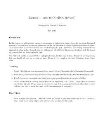
Solved with COMSOL Multiphysics 5.1Laser Heating of a Silicon WaferIntroductionA silicon wafer is heated up by a laser that moves radially in and out over time whilethe wafer itself rotates on its stage. Modeling the incident heat flux from the laser as aspatially distributed heat source on the surface, the transient thermal response of thewafer is obtained. The peak, average, and minimum temperatures during the heatingprocess are computed, as well as the temperature variations across the wafer.10 W laser60 RPMFigure 1: A silicon wafer is heated with a laser that moves back and forth. The wafer isalso being rotated about its axis.Model DefinitionA 2-inch silicon wafer, as shown in Figure 1, is heated for one minute by a 10 W laserthat moves radially inwards and outwards, while the wafer rotates on its stage.Assuming good thermal isolation from the environment, the only source of heat lossis from the top surface via radiation to the processing chamber walls, which areassumed to be at a fixed temperature of 20 C.1 L A SE R H E AT I N G O F A S I L I C O N WA FE R
Solved with COMSOL Multiphysics 5.1The laser beam is modeled as a heat source in the plane with Gaussian profile. To setup the heating profile the model uses the built-in Gaussian Pulse functions, whichenforce that the integral under the curve equals unity. The focal point is moved byusing a triangular waveform to define its position along the x-axis over time. The waferis assigned a bulk rotational velocity in the governing heat transfer equation.The emissivity of the surface of the wafer is approximately 0.8. At the operatingwavelength of the laser, it is assumed that absorptivity equals emissivity. The heat loaddue to the laser is thus multiplied by the emissivity. Assuming also that the laser isoperating at a wavelength at which the wafer is opaque, no light is passing through thewafer. Therefore, all of the laser heat is deposited at the surface.The wafer is meshed using a triangular swept mesh. Swept meshing allows for only asingle thin element through the thickness, and still maintains reasonable element sizein the plane. A finer mesh would give slightly more accurate predictions of the peaktemperature, but predictions of average and minimum temperature would not begreatly affected.Results and DiscussionFigure 2 plots the maximum, minimum, and average temperatures of the wafer, whileFigure 3 shows the difference between the maximum and minimum temperature. Thetemperature distribution across the wafer is plotted in Figure 4.The heating profile does introduce some significant temperature variations, becausethe laser deposits the same amount of heat over a larger total swept area when it isfocused at the outside of the wafer. An interesting modification to this example wouldbe to investigate alternative heating profiles for smoother heating.2 L AS E R H E A T I N G O F A S I L I C O N WA FE R
Solved with COMSOL Multiphysics 5.1Figure 2: Maximum, minimum, and average temperatures of the wafer as functions oftime.Figure 3: Difference between maximum and minimum temperatures on the wafer.3 L A SE R H E AT I N G O F A S I L I C O N WA FE R
Solved with COMSOL Multiphysics 5.1Figure 4: Temperature variation across the wafer. The arrow plot describes the velocity ofthe wafer.Application Library path: COMSOL Multiphysics/Heat Transfer/laser heating waferModeling InstructionsFrom the File menu, choose New.NEW1 In the New window, click Model Wizard.MODEL WIZARD1 In the Model Wizard window, click 3D.2 In the Select physics tree, select Heat Transfer Heat Transfer in Solids (ht).3 Click Add.4 L AS E R H E A T I N G O F A S I L I C O N WA FE R
Solved with COMSOL Multiphysics 5.14 Click Study.5 In the Select study tree, select Preset Studies Time Dependent.6 Click Done.GLOBAL DEFINITIONSStart by defining parameters for use in the geometry, functions, and physics settings.Parameters1 On the Home toolbar, click Parameters.2 In the Settings window for Parameters, locate the Parameters section.3 In the table, enter the following settings:NameExpressionValueDescriptionr wafer1[in]0.0254 mWafer radiusthickness275[um]2.75E-4 mWafer thicknessv rotation60[rpm]1 HzRotational speedangular v2*pi*v rotation6.283 HzAngular velocityperiod10[s]10 sTime for laser to moveback and forthr spot2.5[mm]0.0025 mRadius of laser spot sizeemissivity0.80.8Surface emissivity ofwaferp laser10[W]10 WLaser powerHere, the unit 'rpm' is revolution per minute.GEOMETRY 1Create a cylinder for the silicon wafer.Cylinder 1 (cyl1)1 On the Geometry toolbar, click Cylinder.2 In the Settings window for Cylinder, locate the Size and Shape section.3 In the Radius text field, type r wafer.4 In the Height text field, type thickness.5 L A SE R H E AT I N G O F A S I L I C O N WA FE R
Solved with COMSOL Multiphysics 5.15 Click the Build All Objects button.DEFINITIONSDefine functions for use before setting up the physics.Gaussian Pulse 1 (gp1)1 On the Home toolbar, click Functions and choose Local Gaussian Pulse.2 In the Settings window for Gaussian Pulse, locate the Parameters section.3 In the Standard deviation text field, type r spot/3.The laser beam radius is equal to three standard deviations of the Gaussian pulse.These three standard deviations account for 99.7% of the total laser energy.6 L AS E R H E A T I N G O F A S I L I C O N WA FE R
Solved with COMSOL Multiphysics 5.14 Click the Plot button.Waveform 1 (wv1)1 On the Home toolbar, click Functions and choose Local Waveform.2 In the Settings window for Waveform, locate the Parameters section.3 From the Type list, choose Triangle.4 Clear the Smoothing check box.5 In the Angular frequency text field, type 2*pi/period.6 In the Phase text field, type pi/2.7 In the Amplitude text field, type r wafer.7 L A SE R H E AT I N G O F A S I L I C O N WA FE R
Solved with COMSOL Multiphysics 5.18 Click the Plot button.Analytic 1 (an1)1 On the Home toolbar, click Functions and choose Local Analytic.2 In the Settings window for Analytic, type hf in the Function name text field.3 Locate the Definition section. In the Expression text field, typep laser*gp1(x-wv1(t))*gp1(y).4 In the Arguments text field, type x, y, t.5 Locate the Units section. In the Arguments text field, type m, m, s.6 In the Function text field, type W/m 2.7 Locate the Plot Parameters section. In the table, enter the following settings:8 ArgumentLower limitUpper limitx-r spotr spoty-r spotr spottperiod/4period/4L AS E R H E A T I N G O F A S I L I C O N WA FE R
Solved with COMSOL Multiphysics 5.18 Click the Plot button.Next, add coupling operators for the result analysis.Average 1 (aveop1)1 On the Definitions toolbar, click Component Couplings and choose Average.2 Select Domain 1 only.Maximum 1 (maxop1)1 On the Definitions toolbar, click Component Couplings and choose Maximum.2 Select Domain 1 only.Minimum 1 (minop1)1 On the Definitions toolbar, click Component Couplings and choose Minimum.2 Select Domain 1 only.H E A T TR A N S F E R I N S O L I D S ( H T )Set up the physics. First, include the wafer’s rotational velocity in the governing heattransfer equation.Heat Transfer in Solids 1In the Model Builder window, under Heat Transfer in Solids (ht), click Heat Transfer inSolids 1.9 L A SE R H E AT I N G O F A S I L I C O N WA FE R
Solved with COMSOL Multiphysics 5.1Translational Motion 11 On the Physics toolbar, click Attributes and choose Translational Motion.2 In the Settings window for Translational Motion, locate the Translational Motionsection.3 Specify the utrans vector as-y*angular vxx*angular vy0zNext, add heat flux and surface-to-ambient radiation on the wafer’s top surface.Heat Flux 11 On the Physics toolbar, click Bounda
3.Do the 2 exercises attached at the end of this document. (credit: COMSOL) Objectives and Deliverables The objective of this course is for you to apply concepts and skills in modeling and simulation to problems in biological transport. The objectives of this particular exercise are to gain practice using COMSOL.