Transcription
Towards predicting noise-power-distancecurves for propeller and rotor poweredaircraftAmargianitakis, DC, Self, RH, Proenca, AR, Synodinos, A and Torija Martinez, ds predicting noise-power-distance curves for propeller and rotorpowered aircraftAuthorsAmargianitakis, DC, Self, RH, Proenca, AR, Synodinos, A and TorijaMartinez, AJPublication titleINTER-NOISE and NOISE-CON Congress and Conference Proceedings,InterNoise21, Washington, D.C., USAPublisherInstitute of Noise Control Engineering, USA (INCE-USA)TypeConference or Workshop ItemUSIR URLThis version is available at: d Date2021USIR is a digital collection of the research output of the University of Salford. Where copyrightpermits, full text material held in the repository is made freely available online and can be read,downloaded and copied for non-commercial private study or research purposes. Please check themanuscript for any further copyright restrictions.For more information, including our policy and submission procedure, pleasecontact the Repository Team at: library-research@salford.ac.uk.
Towards predicting Noise-Power-Distance curves for propeller androtor powered aircraftAmargianitakis D.C.1Self R.H.2Proença A.R.3Synodinos A.P.4 , Visiting AcademicInstitute of Sound and Vibration, University of SouthamptonSouthampton, Hampshire, SO17 1BJ, UKTorija A.J.5Acoustics Research Centre, University of Salford, Manchester M5 4WT, UKABSTRACTPropeller and rotor based propulsion systems are the predominant choice of power delivery systemin the upcoming Urban Air Mobility market. Fully electric air-taxis (car sized vehicles with VerticalTake-off and Landing, VTOL, capabilities) concepts are using the benefits of the scalable propertiesof electric motors to distribute propulsor units all over the airframe. The large variety of conceptsand configurations of these vehicles poses a serious issue in predicting noise generated on theground. The need for a high-level model to aid in acoustic decision making is evident. Throughthe demonstrated methodology of computationally deriving Noise – Power – Distance curves forconventional turbo fan aircraft, this paper delivers the capability of dealing with propeller propulsionsystems and the associated propeller tonal noise sources to generate the NPDs and therefore noiseexposure maps. The aims can be broken down into two objectives: a) demonstrate the capabilitiesof the proposed propeller harmonics noise scaling laws to calculate noise variation from a baselinescenario and b) incorporate the scaling components into the larger capability of producing noiseexposure contours, by the means of computationally deriving Noise-Power-Distance curves forpropeller power aircraft. Preliminary NPD curves for General Aviation sized propeller poweraircraft are generated and ijaMartinez@salford.ac.uk
1.NOMENCLATUREqSYMBOLSMr ΩMtΩrt /c0 , tip rotational Mach numberMx V/c0 , flight Mach numbern mB harmonic of shaft frequencyppressure disturbancePncomplex Fourier coefficient of prDistance from origin to observer2π times the shaft rotation frequencyΨV , ΨD , ΨL normalised source transformsM x2 z2 Mt2 section relative Mach numberθradiation angle from propeller axisBnumber of bladesBD b/D, chord-to-diameter ratioCDdrag coefficientCLlift coefficientDpropeller diameterrt D/2 propeller tip radiusJnBessel functiontbratio of maximum thickness to chordk x , kywave numbersVflight speedmharmonic of blade passing frequencyq M x2 Mt2 helical tip Mach numberyobserver distance from propeller axisz r0 /rt normalised radial coordinateMh2.INTRODUCTIONThe Urban Air Mobility (UAM) market [1] is quickly taking over a major part of research withinthe aeronautic and aviation industry. While simultaneously investors and financial researchers areevaluating the market growth could create a 1.5 trillion market by 2040 [2], with evidence lying inthe fact that major airlines placing orders of billions worth of electric vertical take-off and landing(VTOL) aircraft.Many designers are choosing propeller and rotor propulsion systems alongside fully orhybrid electric energy storage and delivery systems. As an inevitable consequence the study ofpropeller/rotor noise is regaining the interests of research organisations. The major noise generatingmechanisms are basically the same for all rotating blades, whether that be propellers or rotors. Thesemechanisms can be further broken down into discrete frequency noise (thickness, loading, etc) andbroadband components with the relative importance of each depending on design and operatingconditions.In a greater attempt to model the noise of these novel aircraft and their operations in the Instituteof Sound and Vibration (ISVR), this paper initiates the development of a framework able to carryout high-level assessment of UAM vehicles early in the design process, when limited input datais available. There is an obvious necessity for tools able to carry out multiple studies at lowcomputational cost to 1. enable the exploration of a large design space in terms of noise outputearly in the decision-making process and 2. provide crucial information to manufacturers about theacoustic impact their vehicle will have in the community of operation.This paper focuses on the purely computational generation of Noise-Power-Distance (NPD) curvesof propeller/rotor powered aircraft. NPD curves could then be coupled with traditional airport noisemodels such as the FAAs AEDT [3] and Eurocontrol’s tool IMPACT [4] or high level communitynoise models such as RANE [5] to calculate noise maps (contours). The framework is based on theknowledge of baseline noise levels of an appropriately chosen baseline aircraft. Then using individualnoise source prediction scaling laws for the dominant sources of sound, changes to the sound power
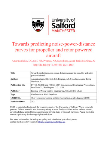
output, between the baseline and study aircraft are evaluated. Once the initial points of the LA,maxNPDs are calculated, the standard SAE AIR 1845 [6] computational procedure is used to extrapolateto all other NPD distances. SEL NPDs are then also computationally generated by implementingflyovers of a lumped source model comprised of said dominant sources. Finally, to demonstrate thecapability of the model, preliminary NPDs for two current propeller aircraft are generated; a singlereciprocating engine powered Cessna 172 and the twin engine turboprop de Havilland Canada DHC-6Twin Otter.3.REVIEW OF HANSON FREQUENCY DOMAIN MODEL FOR PROPELLERHARMONIC NOISEThe development of scaling laws in many cases depends on experimental measurements and datacollected for specific sources and operations parameters. These are laws based on empirical or semiempirical models and have proved to be a reliable way of predicting the acoustic field for variousaeroacoustics sources; some of these include, fan noise [7], jet noise [8] and airframe noise [9] . Inthis paper, a simplified version of the frequency domain method developed by Hanson is derived, withthe intention of understanding the underlying physics connecting the noise output and key parameters.Figure 1: Geometry of rotating source and acoustic field.As previously mentioned steady loading and thickness noise sources constitute the linear contentof the sound field that can be modelled by the linearised equations of motion for an inviscid fluid. TheHanson model is a far-field frequency domain model for a single rotating propeller using a helicoidalsurface representation of the blades. Hanson’s formulation was chosen in this study as it accounts forthe linear thickness and loading sources and the nonlinear quadrupole sources (although emitted dueoperation regime) including forward flight, and to this day represents a unifying theory of propellerharmonic noise. Hanson published an extension to the method to account for unsteady-loading whichwill be omitted for the analysis presented within this paper but will be considered in future work.Hanson’s derivation starts at the Goldstein version of the acoustic analogy,!Z TZZ TZ G G1 2G10ρ0 Vn fidτ 2Ti jdydτ(1)ρ (x, t) 2 τ yic0 T S (τ)c0 T ν(τ) yi y jAn approximation from thin wing aerodynamic theory is used, permitting the surface boundaryconditions to be satisfied on a mean surface rather than on the blade upper and lower surfaces. Thus,the source strengths Vn and fi are determined from actual blade geometry but their point of action ison the mean helicoidal surface (To be further discussed in the asymptotic approximation Section 4).For B blades, the mth harmonic of blade passing frequency is found by setting n mB andmultiplying by Ω. Waveforms can be computed from the Fourier series. To study the effects ofblade design and operation parameters Hanson recast his solution into a form that explicitly displays
these variables. This form is duplicated here for the ease of the reader and is the starting point of theasymptotic analysis and scaling model within this paper: ih PπΩr2Vm ρcBsinβexpimB 00c02 PDm 8π y/D 1 M x cos β PLm Z1Mr2 exp (iφ s )JmB 0 2 ktΨ(k)! bVx x mBzMt sin β dzik(C/2)Ψ(k) xDD x 1 M x cos β iky (C L /2)ΨL (k x ) (2)with φ s representing a phase lag due to blade sweep (neglected further on in this study as simpleblade geometry is assumed), while k x and ky being dimensionless wave numbers defined by,kx 2mBBD MtMr (1 M x cos θ)(3)2mBBD M x Mr2 cos θ ky (4)zMr1 M x cos θIn this form, ΨV ,ΨD and ΨL represent the Fourier transforms of the three sources giving thethickness and loading distributions of the blade, 1 2 H(x)Ψ(k)ZVx exp (ik x x)dx(5) f(x)Ψ(k) DD x ΨL (k x ) 1 fL (x) 2Finally the contributions of the individual sources may be summed to get the Fourier transformcoefficient of the pressure at the mth harmonic of the blade passing frequency PmB , while the far-fieldtime domain pressure may be given Fourier transform itself.4.SCALING OF PROPELLER HARMONIC NOISEThe use of analytical formulas for the derivation of scaling laws is advantageous as direct insightto the influence of design geometry and operating conditions have on the fundamental and itsharmonics, may be accomplished without full scale experimental procedures. Literature suggeststhat for propeller harmonic noise not single global scaling law exists (such as Lighthill’s eighthpower law for jet noise) and rather analytical time or frequency domain models may be used (withthe disadvantage a slight increase in time, computational power and inputs requirement) to get muchmore accurate estimation of the sound power (total acoustic energy) emission [10].Some of the main assumptions of the Hanson frequency domain model will be transcribed here, asthe applicability and limitation range of the approximations and scaling laws will directly correlateto starting model. The problem is treated assuming propeller in flight with uniform flow. The sourceterms used in the derivation are, the monopole (volume), dipole (loading) and quadrupole (Lighthill’sstress tensor neglecting viscosity), however the quadrupole term is ignored as it becomes significantat transonic blade section speeds [11] (general aviation applications generally consider a maximumblade tip mach number of 0.8 or Mt 0.8). The "thin-blade" approximation permits the mathematicalsimplification of replacing the blade surfaces by their effect on the fluid, this results in errors only atvery high harmonic order, and out of the plane of rotation. Finally, Doppler factors in both amplitude
and frequency roles are contained with the model, although the relatively low cruise speeds of generalaviation vehicles in question are not strongly affected.The Bessel function makes an appearance in all harmonic noise terms PVm , PDm and PLm , it largelycontributes to the spectral shape of the radiated noise and the overall level and is sometimes referredto a "radiation-factor". The argument mBzMt sin β/(1 M x cos β) takes maximum values within theplane off rotation, that is β 90o , and is equal to mBzMt . For tip Mach numbers applicable togeneral aviation vehicles the argument mBzMt remains approximately equal (or slightly smaller) tothe order mB of the Bessel functions where its value peaks. This behaviour may be approximatedusing the small argument asymptotic formula. For the ease we introduce the variable α1 where α1 sin β/(1 M x cos β), therefore the asymptotic approximation of the Bessel function in Equation 2 maybe given by,!mB mBMt α11(6)JmB mBMt α1 (mB)!2The source terms (the terms in braces of the integral in Equation 2) may be broken down intoterm in two components: a Spectrum shape component and a spectrum level component. The Ψterms represent the effect of chordwise noncompactness, that is, interference at the observer locationof signals emitted from various source locations along the chord, contributing to the spectrum shapedefinition. Chordwise blade geometry and loading is what determines these characteristics, thereforewe assume a simple parabolic thickness distribution and uniform lift and drag distribution. Thethickness, drag, and lift noise components are directly proportional to the thickness ratio tb , dragcoefficient C D , and lift coefficient C L , respectively. Combining the noncompactness effect relationalong with the proportionality we may estimate the source term transforms by,1 M x sin θ1ΨV (k x ) 2 kx2mBBD Mt!211 M x sin θΨD (k x ) ΨL (k x ) kx2mBBD Mt(7)!(8)Therefore the individual source contributions may be estimated as simple functions of the bladethickness, tb and blade loading, C L and C D ,k2x tb ΨV (k x ) tb(9)k x (C D /2)ΨD (k x ) C D /2(10)C L ky (M x Mh2 cos θ) C L (11)2k xMt2The dominating term within the integral in the radial direction is the square of the section relativeMach number, Mr2 . The section relative Mach number take maximum at the tip of the propeller, andis equal to the helical Mach number Mh . We may estimate the value of the integral by assuming it isdirectly proportional to Mh2 , and for a static case proportional to Mt2 , as can be seen,k x (C L /2)ΨL (k x ) Mr2 Mh2 M x2 Mt2(12)This assumption implies that the thickness and loading sources are applied on the propeller tipsection. To correct the thickness and loading parameters to account for the entire blade we assumethe thickness ratio at the blade tip takes the average value over the blade, tb (z 1) t b , and the loadingcoefficient follow accordingly, C D (z 1) C D and C L (z 1) C L (Note: the loading parameters
C D and C L may instead be defined in terms of thrust and torque, dT/dz and dQ/dz respectively, withthe integral over the radius giving the thrust and torque acting on the blade).Combining of the above mentioned procedures and adding the contributions of the individualsources together we may estimate PmB PVm PDm PLm as,PmBρ0 c20 8π!!!!!mBDsin θ1mBMt sin θ2My (1 M x cos θ) h (mB) 2(1 M x cos θ) C D C L (M x Mh2 cos β) t b 22MtΩr π exp imB c02"(13)!#As we are interested in the sound power output as a function of design and operational parameterwe must first estimate the intensity which is proportional to p2rms , therefore we have, 2!2!2 ρ0 c201C D C L (M x Mh2 cos β) 2 2 4 pm,rms hPmB PmB i D Mh t b 8πy22Mt {z} {z } {z}constants Spherical Spreadingsin θ (1 M x cos θ) {zDirectivityDesign/operation parameters!4mB 2!2!2mB1mBMt(mB)!2} {z}(14)Spectral ShapeThe asymptotic approximation allows for some simple observations to be made regarding theinfluence of the tip Mach number. Assuming as previously, Mt 1 the Mt2mB term in Equation14 shows that at a given rotation rate propellers with larger blade number generate less sound andfurthermore the contribution of the higher harmonics rapidly decreases with increasing harmonicorder m while the tip rotation speed remains subsonic. This allows for a modelling technique usedby Heidmann for the estimation of fan discrete-tone and combination-tone noise [7], to be applied.The procedure involves predicting the spectrum level and spectrum shape. The spectrum level isdefined at each design/operation point by the fundamental tone, while the levels of remaining spectralfrequencies are estimated by referencing the blade passing frequency and the spectral shape function.However, unlike Heidmann the spectrum shape is not constant, rather a function of the blade numberand tip mach number.The sin θ present within the Bessel function argument, and therefore in the approximation relation,causes highly documented dipole behaviour of the propeller. The radiated noise diminishes towardsthe propeller axis as approached from both front and rear directions. Additionally, the Doppler factor1 M x cos β) causes a shift of that directivity pattern into the forward hemisphere with respect to thepropeller plane.The overall sound power output of the system may therefore be evaluated through the averageintensity emitted over angles β and ϕ, which may be evaluated in the far field through the root-meansquare,4πR2W 4πR I ρ0 c0Z2π Zπ2 00p2rms R2 sin β dβdϕ(15)
The calculation of I pressure depends on the integration over the spherical surface surrounding thesource. The integral over ϕ takes a trivial answer as rotational symmetry exists around the propelleraxis. When considering the evaluation of the integral over the polar angle β over in the intervalβ (0, π) the solution is no longer trivial. The problem may be divided into two cases, a. a static(or hovering) propeller, meaning M x 0 and b. the case where mean flow is non-zero, M x , 0 andassuming subsonic flight speeds (M x 1).The evaluation for the two cases are omitted for terseness, and will included in future publications.In addition the methodology following in Section 5 allows for calculation of the variation ofsound power emitted including directivity effects, therefore the overall sound energy quantificationbypassed.5.NOISE VARIATION DUE TO CHANGESTo incorporate the effect of changing engine power settings, the derived equations are functionsof propeller and aircraft operational parameters (thrust setting, torque, rpm e.t.c.) that vary betweenoperational procedures.It has been previously demonstrated that the use of changes in noise, or PWL, as comparedto a baseline scenario gives more accurate prediction than attempting to evaluate absolute valuesdirectly using the scaling laws. Coupled with the capability of using PWL in order to generateNoise-Power-Distance curves the use of the scaling formulation may be extended to computationallyevaluating modified rotor designs in an urban airport environment through the use of exposure metricsand contours.Figure 2: Diagram of typical flyover procedure for obtaining NPD data.The basis of this methodology assumes that any noise level (PWL) of the subject ( modified )aircraft is given in terms of the sum of a baseline aircraft noise level and the difference in noise levelbetween the two aircraft,Considering a baseline aircraft, it consists of noise sources emitting overall sound power W0 . As aresult of operational or technological changes, the acoustic noise sources on the aircraft may changein number, magnitude and other acoustic properties, e.g. spectral content, therefore denoting n thetotal number of noise sources after the modifications and s an individual noise source that changed byacoustic power W s we may write,nXW W0 W s(16)s 1noting that for noise sources that previously did not exist, W s W s and for sources that wereremoved, W s W s . Therefore in order to calculate the acoustic emission of the novel aircraftdesign, knowledge on the acoustic output of the baseline aircraft is required, along with the individualchanges of the acoustic sources. As mentioned, Synodinos [12] demonstrated this methodologyfor jet, fan and airframe noise sources on conventional turbofan aircraft, and applied it on novel
ducted fan configurations (considering the same acoustic sources [13]). Following we will extendthe methodology to incorporate the propeller harmonic noise sources though the use of scalingexpressions developed in the previous sections. The methodology includes an elegant way ofincluding the tonal spectral content of propeller noise when calculating the change in noise( Noise)between configurations. This is achieved through the use of a spectral shape function. In this paper, aspectral shape function is explored through the use of the scaling expressions and therefore a productof the starting Hanson model, however other functions may be used to define the spectral contentshape according to the application.The remaining part of this section is dedicated to deriving the change in noise (or specificallythe change in SPL) emitted by a propeller aircraft, considering loading and thickness noise sources.The propeller discrete tone noise (as it pertains to the mentioned sources) of any aircraft may beexpressed as the energy sum across all harmonics. The individual harmonic levels may be related tothe fundamental tone by some spectra shape function, allowing for the SPL to be written as, X L F f /10 (17)L p,0 10 log10 10 f1 ,0 1 f1 ,0 m 1with f mBΩ and f1 BΩ represent the frequency of mode m and the fundamental tone respectively,while L f1 ,0 is the SPL of the baseline fundamental. F1 denotes the spectra shape function.When modifications in terms of operational and/or design parameters are made, changes to thefundamental tone, L f1 and the shape of the harmonics F1 are observed, leaving the new SPL as, X L F f L F f /10 1 ff1 1(18)L p 10 log10 10 f1 ,0 1 f1 ,0 m 1where L f1 L f1 ,0 L f1 represents the new level of the fundamental tone, and Lm ( f ) L f1 F1 ( f / f1 ) represents the new sound level of the harmonics (narrowband spectrum).Returning to Equation 14, we may consider a case where modifications to a baseline aircraft aremade. The change in level of the fundamental frequency observed may be estimated by setting m 1in both cases and taking the difference between the two, leaving, 2 p f (19) L f1 10 log10 2 1 p f1 ,0or!!!yBDMh L f1 20 log10 20 log10 40 log10y0B0 D0Mh0 20 log10 20 log10tb C D /2 C L (M x Mh2 cos β)/(2Mt )!(20)2tb,0 C D,0 /2 C L,0 (M x,0 Mh,0cos β0 )/(2Mt,0 )!!![sin β/(1 M x cos β)]2B 1B0 !(BMt )B 20 log10 20 log10B!B0 Mt,0 )B0[sin β0 /(1 M x,0 cos β0 )]2B0 1where the subscript 0 denotes the values corresponding to the condition before the modifications wereapplied (baseline).Separating all terms including the mode number m in Equation 14 we may define a function S .This function determines the shape of the harmonics.sin βS (m) 1 M x cos β!4mB 21(mB)!!2mBMt2!2mB(21)
Normalising this expression by its value for m 1,S (m)sin βf(m) f1S (1)1 M x cos β!4B(m 1)B!(mB)!!2BMt2!2B(m 1)m2mB(22)noting that ff1 (1) 1 by definition. Finally the change in level of the harmonics (m 1) between abaseline case and a modified counterpart may be given by, F1!!!B!(mB0 )!fmB 20m log10 B0 20 log10f1mB0 !(mB)!(23) 20 log106.!!(BMt )B(m 1)[sin β/(1 M x cos β)]B(m 1) 40 log10(B0 Mt,0 )B0 (m 1)[sin β0 /(1 M x,0 cos β0 )]B0 (m 1)NOISE-POWER-DISTANCE CURVE GENERATIONThis section presents the methodology of computationally generating NPDs using the knowledgeof how propeller noise changes as a function of changes in the design and operational parameters.The same approach to the derivation of computational NPDs can be seen in [12], where NPDs for fan,jet and airframe noise sources were calculated. The work in this section is novel with regards to thepropeller noise sources, and aims on extending the methodology presented in said publications.The steps in producing NPD curves for propeller powered aircraft from a baseline measured NPDpoint and aircraft noise variation due to design or operational changes are almost identical to thatof conventional aircraft, although differences do occur in the treatment of the spectral content of thesound levels, as changes to the discrete tonal content are also accounted for by the propeller scalingmodel. For brevity reasons a detailed explanation is omitted but is intended for future publications.For detailed explanation the reader is encouraged to follow the procedure described in [12] and [14]along with the SAE AIR1845 [6] computational step.7.PRELIMINARY NPDS FOR PROPELLER POWERED AIRCRAFTIn order to validate while at the same time demonstrating the capability of the scaling laws inconjunction with the PWL methodology, this section estimates both LA,max and SEL NPD curves oftwo different propeller powered aircraft and compares to published data [15].For each aircraft a baseline point is chosen (depicted with a red cross in Figures 3 and 4, thispoint corresponds to a specific power setting j and slant distance d) on the LA,max curves, accordingto the type of operation of interest. Using the single baseline value and the methodology described inSections 4, 5 and 6 predictions for the rest of the NPD slant distances and power setting are made. Thefirst validation case is the Cessna 172 (Maximum take-off weight (MTOW) 1,114 kg). The chosenNPD point corresponds to that of slant distance equals 304.8 m (or 1,000 ft). Figure 3 show thedeparture NPDs for the Cessna 172 at two specific power setting; 59.6% and 100% of maximumstatic thrust (MST) respectively. The published data may be seen in dashed lines, while the predictedin solid ones.The second validation case demonstrates the capability of estimating NPD for slightly larger turboprop (MTOW 5,682 kg, still within the "small" noise category of aircraft defined by the ICAO Annex16 [16]) with a twin engine configuration. Figure 4 compares the published and predicted take-offNPD curves (using same notation) at this time 30% and 100% of MST.
040005000600070008000010002000(a) LA,max300040005000600070008000(b) SELFigure 3: Published and predicted departure NPDs for a single engine Cessna 172 0002000300040005000(a) 0(b) SELFigure 4: Published and predicted departure NPDs for twin engine de Havilland Canada DHC-6 (TwinOtter)8.CONCLUSIONSThe work presented within this paper summarises the methodology of computing NPD curvesfor propeller/rotor power aircraft. A scaling law of the dependence of the fundamental tone of theharmonic noise due to thickness and loading source is coupled with a spectral shape function to fullydefine the discrete tonal content of a propeller source. Using a reference baseline, the change inoverall noise output due to changes in propeller parameters is calculated. This change in noise is thenused to computationally derive Noise-Power-Distance curves, which serve as the main input for noiseexposure map models.The validation / case studies presented within this paper represent initial results that are tied to afew significant simplification assumptions. Namely a) both types of NPD curves presented (LA,maxand SEL) are strongly dependant to the overall directivity of the aircraft. In this initial study theassumption of a simple dipole source directivity was made. This assumption is closely related to thenext assumption discussed, that of a single dominant acoustic noise source. The aircraft is representedby the assumed dominant propeller tonal noise. Propeller tonal noise due to loading and thicknesssource as discussed by Hanson in [17], [18], [19] and others [20], [21]. Realistic directivity dataof propeller aircraft flyovers could potentially reduce the error in both types of NPD curves. b)the propeller and specifically propeller tonal noise is assumed to be the dominant source. As of
this preliminary study this assumption results in the negligence of other possible aeroacoustic noisesources (e.g. airframe noise, reciprocating engine noise, jet noise etc. ) that may be present. Thisassumption may be justified for takeoff procedures as high thrust requirements lead to heavily loadedpropeller blades contributing to the discrete loading noise. However, approach procedures may sufferfrom the opposite effect of low loading characteristics. Therefore future approach calculations willconsider addition model to account for airframe noise etc, as in [12]. In the case of the Cessna 172,the reciprocating engine noise is assumed to be effectively masked by the propeller noise [22]. Thesame hold for turboprop engine architectures as in the case of the DHC-6, where the combustion andjet noise sources are considered negligible with respect to the propeller source [23]. Finally, c) thefinal point of discussion brings two points into one. The frequency content of the predicted NPDcurves depends on two factors, 1. the baseline spectra and 2. the predicted changes to the spectraby the scaling model. Baseline spectral data (specifically spectral shapes) for different operationalregimes are not readily available. The predictions within this paper are based on spectral shapes offlyover measurements at the highest possible power setting (100 % MST). The predicted changes tothe spectra may also lead to errors as discrete-tonal noise of the propeller is only accounted for (e.g.changes in high-frequency vortex broadband noise are not captured). As mentioned closely coupledwith the frequency content of the sound in the atmospheric attenuation. As the attenuation is relatedto the propagation distance and the frequency of the sound, the large NPD slant distances tend toamplify the error associated with the prediction of the spectra shape change.Nevertheless, despite the sources of error discussed, th
x;k y wave numbers m harmonic of blade passing frequency M h q M 2 x M t helical tip Mach number M r q M 2 x z2M t section relative Mach number M t r t c 0, tip rotational Mach number M x V c 0, flight Mach number n mB harmonic of shaft frequency p pressure disturbance P n complex Fourier coe cient of p r Distance from origin to .