Transcription
NBER WORKING PAPER SERIESTHE MARKET FOR CRASH RISKDavid S. BatesWorking Paper 8557http://www.nber.org/papers/w8557NATIONAL BUREAU OF ECONOMIC RESEARCH1050 Massachusetts AvenueCambridge, MA 02138October 2001The views expressed herein are those of the author and not necessarily those of the National Bureau ofEconomic Research. 2001 by David S. Bates. All rights reserved. Short sections of text, not to exceed two paragraphs, maybe quoted without explicit permission provided that full credit, including notice, is given to the source.
The Market for Crash RiskDavid S. BatesNBER Working Paper No. 8557October 2001JEL No. G13ABSTRACTThis paper examines the equilibrium when negative stock market jumps (crashes) can occur, andinvestors have heterogeneous attitudes towards crash risk. The less crash-averse insure the morecrash-averse through the options markets that dynamically complete the economy. The resultingequilibrium is compared with various option pricing anomalies reported in the literature: the tendency ofstock index options to overpredict volatility and jump risk, the Jackwerth (2000) implicit pricing kernelpuzzle, and the stochastic evolution of option prices. The specification of crash aversion is compatiblewith the static option pricing puzzles, while heterogeneity partially explains the dynamic puzzles.Heterogeneity also magnifies substantially the stock market impact of adverse news about fundamentals.David S. BatesFinance DepartmentUniversity of IowaIowa City, IA 52242-1000and NBERTel: 319-353-2288Email: david-bates@uiowa.edu
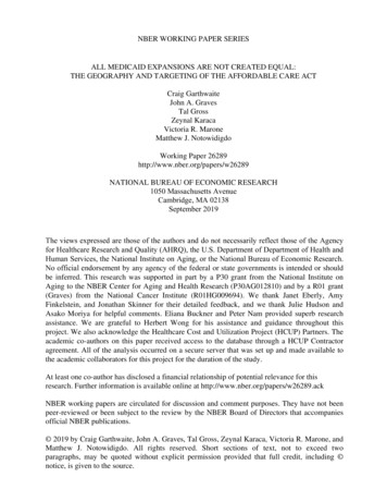
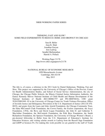
Empirical option pricing research involving stock index options has revealed substantial divergencesbetween the “risk-neutral” distributions compatible with observed post-’87 option prices, and theconditional distributions estimated from time series analyses of the underlying stock index. Perhapsthe most important has been the substantial disparity between implicit standard deviations (ISD’s)inferred from at-the-money options, and the subsequent realized volatility over the lifetime of theoption. As illustrated below in Figure 1, ISD’s have generally been higher than realized volatility.Furthermore, regressing realized volatility upon ISD’s almost invariably indicates that ISD’s areinformative but biased predictors of future volatility, with bias increasing in the ISD level.While the level of at-the-money ISD’s is puzzling, the shape of the volatility surface acrossstrike prices and maturities also appears at odds with estimates of conditional distributions. It is nowwidely recognized that the “volatility smirk” implies substantial negative skewness in risk-neutraldistributions, and various correspondingly skewed models have been proposed: implied binomialtrees, stochastic volatility models with “leverage” effects, and jump-diffusions. And although thesemodels can roughly match observed option prices, the associated implicit parameters do not appearespecially consistent with the absence of substantial negative skewness in post-’87 stock indexreturns. To paraphrase Samuelson, the option markets have predicted nine out of the past fivemarket corrections. A further puzzle is that the predictions are somewhat countercyclical. Withinthe Bates (2000) jump-diffusion model, implicit jump risk was highest immediately after substantialmarket drops, and was low during the bull market of 1992-96.It is of course possible that the pronounced divergence between objective and risk-neutralmeasures represents risk premia on the underlying risks. The fundamental theorem of asset pricingstates that provided there exist no outright arbitrage opportunities, it is possible to construct a“representative agent” whose preferences are compatible with any observed divergences betweenthe two distributions. However, Jackwerth (2000) and Rosenberg and Engle (2000) have pointedout that the preferences necessary to reconcile the two distributions appear rather oddly shaped, withsections that are locally risk-loving rather than risk-averse. Furthermore, the post-’87 Sharpe ratiosfrom writing put options or straddles seem extraordinarily high -- two to six times that of investingdirectly in the stock market.
2The overall industrial organization of the stock index option markets does not appearespecially compatible with the idealized construction of representative agents. In that construction,all individuals trade until at the margin they are indifferent to taking on more or less risk. Theresultant risk-pooling of systematic risks across all agents permits the calibration of standard assetpricing models from aggregate data sources: e.g., estimating the consumption CAPM based onaggregate consumption data, or the CAPM based on proxies for the return on aggregate wealth.However, most investors do not routinely use options to manage the underlying risks. Althoughstock index options are among the most actively traded options, the stock positions hedged byexchange-traded options on the S&P index or futures represented at most 2.6% of the S&P 500market capitalization in 1998.1In stock index option markets, individual investors can easily buy options but face obstaclesat the broker level to writing naked puts or calls. While hard data are not readily available,anecdotal evidence suggests a fundamental post-’87 dichotomy between the buyers and sellers inthe stock index option market. A broad array of individual and institutional investors buy optionsas part of their overall risk management strategies, while a relatively concentrated group of optionmarket makers predominantly write them and delta-hedge their positions. And although all investorsneed not be rational for markets to be efficient, this broad and apparently persistent dichotomybetween buyers and sellers suggests closer scrutiny of option market making is warranted.The objective of this paper is therefore to focus more carefully on the financial intermediation of crash risk through option markets. A general equilibrium model is constructed in whichrelatively crash-tolerant option market makers insure crash-averse investors. Heterogeneity inattitudes towards crash risk is modeled via heterogeneous state-dependent utility functions similarto those in Ho, Perraudin and Sørensen (1996). Crashes can occur in the model, given occasionaladverse jumps in news about fundamentals. Derivatives are consequently not redundant in the1This is computed based upon the 1998 open interest for CBOE options on the S&P 100 andS&P 500 indexes, and for CME options on S&P 500 futures. It represents an upper limit inassuming every option corresponds one-for-one to an underlying stock position. Strategiesinvolving multiple options (vertical spreads, collars, straddles, etc.) would substantially reduce theestimate of the stock positions being protected.
3model and serve the important function of dynamically completing the market. Given completemarkets, equilibrium can be derived using an equivalent central planner’s problem, and thecorresponding dynamic trading strategies and market equilibria are identified.The view of options markets as an insurance market for crash risk may be able to explainsome of the option pricing anomalies -- especially if there exist barriers to entry. If crash risk isconcentrated among option market makers, calibrations based upon the risk-taking capacity of allinvestors can be misleading.2Speculative opportunities such as writing straddles becomeunappealing when the market makers are already overly involved in the business. Furthermore, thedynamic response of option prices to market drops resembles the price cycles observed in insurancemarkets: an increase in the price of crash insurance caused by the contraction in market makers’capital following losses.3This paper therefore represents an initial exploration of the financial intermediation of crashrisk via the options markets. Section 1 recapitulates the various stylized facts from empirical optionsresearch that the various models will attempt to match. Section 2 introduces the basic framework,and identifies a benchmark homogeneous-agent equilibrium. Section 3 explores the implicationsof heterogeneity in agents. Section 4 concludes.2Basak and Cuoco (1998) make a similar point regarding calibrations of the consumptionCAPM when most investors don’t hold stock.3Froot (2001, Figure 3) illustrates the strong, temporary impacts of Hurricane Andrew in1992 and the Northbridge earthquake in 1994 upon the price of catastrophe insurance.
41. Empirical option pricing anomalies and stylized factsThree categories of discrepancies between objective and risk-neutral measures will be kept in mindin the theoretical section of the paper: volatility, higher moments, and the implicit pricing kernelthat in principle reconciles the objective and risk-neutral probability measures. Furthermore, eachcategory can be decomposed further into average discrepancies, and conditional discrepancies.The unconditional volatility puzzle is that implicit standard deviations (ISD’s) from stockindex options have been higher on average over 1988-98 than realized volatility over the options’lifetimes. For instance, ISD’s from 30-day at-the-money put and call options on S&P 500 futureshave been 2% higher on average than the subsequent annualized daily volatility over the lifetimeof the options.4 This discrepancy has generated substantial post-’87 profits on average from writingat-the-money puts or straddles, with Sharpe ratios two to six times that of investing in the stockmarket. See, e.g., Fleming (1998) or Jackwerth (2000).The conditional volatility puzzle is that regressing realized volatility upon ISD’s generallyyields slopes that are significantly positive, but significantly less than one. For instance, theregressions using the 30-day ISD’s and realized volatilities mentioned above yield volatility andvariance results365T22jτ ' t%1 ( ln Fτ ) ' .0160 % .756 ISDt % gt%T , R ' .45(.0142) (.102)T365222j ( ln Fτ ) ' .0027 % .681 ISDt % gt%T , R ' .33T τ ' t%1(.0033) (.161)(1)T4(2)The puzzle is slightly exacerbated by the fact that at-the-money ISD’s are in principledownwardly biased predictors of the (risk-neutral) volatility over the lifetime of the options.
5Figure 1. ISD’s and realized volatility, 1988-98. ISD’s are from 30day S&P 500 futures options. Realized volatility is annualized, fromdaily log-differenced futures prices over the lifetime of the options.with heteroskedasticity-consistent standard errors in parentheses.5 Since intercepts are small, theregressions imply that ISD’s are especially poor forecasts of realized volatility when high.The skewness puzzle is that the levels of skewness implicit in stock index options aregenerally much larger in magnitude than those estimated from stock index returns -- whether fromunconditional returns (Jackwerth, 2000) or conditional upon a time series model that captures salientfeatures of time-varying distributions (Rosenberg and Engle, 2000). Furthermore, implicit skewnessfalls off only slightly for longer maturities of stock index options of, e.g., 3-6 months.6 By contrast,5Christensen and Prabhala (1998) argue that measurement error in ISD’s may be biasingslope estimates downwards, and estimate essentially unitary slopes on post-’87 monthly data usinginstrumental variables. Using instrumental variables on my data had negligible effect on pointestimates. However the associated loss of power did increase standard errors, to the point whereunbiasedness could not be rejected in some cases. Jorion (1995) provides a Monte Carlo assessmentof measurement error’s impact on volatility regressions.6In options research, implicit skewness is roughly measured by the shape of the volatility“smirk,” or pattern of ISD’s across different strike prices (“moneyness”). The skewness/maturityinteraction can be seen by examined by the volatility smirk at different horizons conditional uponrescaling moneyness proportionately to the standard deviation appropriate at different horizons. See,
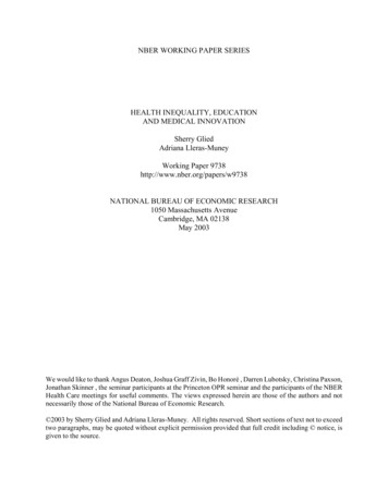
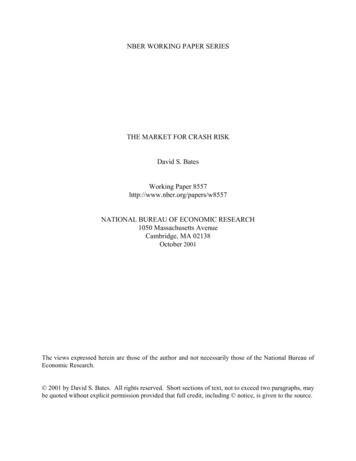
6the distribution of log-differenced stock indexes or stock index futures converges rapidly towardsnear-normality as one progresses from daily to weekly to monthly holding periods.A further puzzle is the evolution of distributions implicit in option prices. Figure 2 belowsummarizes that evolution using updated estimates of the Bates (2000) 2-factor stochasticvolatility/jump-diffusion model with time-varying jump risk. The affine structure of that modelpermits a factor representation of implicit cumulants in terms of two underlying state variables. Thefirst factor (V1) affects variance directly and also determines the jump intensity, thereby affectingcumulants at all maturities. The second factor (V2) influences instantaneous variance (with roughlyTable 1Implicit jump parameters, and (risk-neutral) cumulants at 1- and 6-month horizons,1988-98 estimates.Average jump size:-6.6%Jump standard deviation:11.0%Jump intensity:λt ' 81.41 V1t % .01 V2t1-month cumulantsK2 '1.76e&4 % .2053V1 t % .0795 V2 tK3 ' &1.01e&5 & .0371V1 t & .0012 V2 tK4 ' 2.47e&6 % 10.54e&3 V1 t % .06e&3 V2 t6-month cumulantsK2 ' .0058 % 1.3080 V1 t % .3802 V2 tK3 ' &.0012 & .8112 V1 t & .0336 V2 tK4 ' .0007 % .7556 V1 t % .0083 V2 tAverage factor realizations: Avg(V1 ) ' .0092; Avg(V2 ) ' .0143.3/22Conditional variance K2 ; skewness K3 / K2 ; excess kurtosis K4 / K2 .e.g., Bates (2000, Figure 4). Tompkins (2000) provides a comprehensive survey of volatility surfacepatterns, including the maturity effects.
7Figure 2. Implicit factor estimates from S&P 500 futures options, 1988-98.V1 affects all cumulants, at all maturities. V2 affects conditional variance but has littleimpact on higher cumulants. Units are in instantaneous variance per year conditional on nojumps (left scale), or in implicit jump frequency (right scale). See Bates (2000) forestimation details.half the variance loading of V1 -- see Table 1 below), but has relatively little impact on highercumulants.The graph indicates that the sharp market declines over 1988-98 (in January 1988, October1989, August 1990, November 1997, and August 1998) were accompanied by sharp increases inimplicit jump risk. The puzzles here are the abruptness of the shifts (Bates (2000) rejects thehypothesis that implicit jump risk follows an affine diffusion), and the magnitudes of implicit jumprisk achieved following the market declines. Furthermore, affine models assume the risk-neutral andobjective jump intensity are proportional. These models therefore imply objective crash risk ishighest immediately following crashes, which some (e.g., Chernov et al, 1999) would findunappealing.
8Finally, there is the implicit pricing kernel puzzle discussed in Jackwerth (2000) andRosenberg and Engle (2000). The sharp discrepancy between the negatively skewed risk-neutraldistribution and roughly lognormal objective distribution at monthly horizons causes the risk-neutralmode to be to the right of the estimated objective mode, even though the risk-neutral mean isperforce to the left of the objective mean. If the level of the stock index is viewed as a reasonablygood proxy for overall wealth of the representative agent, this discrepancy in distributions impliesmarginal utility of wealth is locally increasing in areas – implying utility functions that are locallyconvex in areas, rather than globally concave.7It is possible that a standard representative agent/pricing kernel model can explain the abovepuzzles. Pan (2001), for instance, finds a substantial risk premium on time-varying jump risk is apromising candidate. The risk premium raises implicit jump risk, volatility, and skewness relativeto the values from the objective distribution, while the time variation in jump risk can explain theconditional volatility bias. Bates (2000) finds that this model can also match the maturity profileof implicit skewness better than models with constant implicit jump risk.The challenges for this explanation are the magnitude of the speculative opportunitiesassociated with the implicit risk premia, and its failure to address the pricing kernel anomaly. Thestochastic evolution of implicit and objective jump risk is also puzzling,7Jackwerth’s results are disputed by Aït-Sahalia and Lo (2000), who find no anomalies whencomparing average option prices from 1993 with the unconditional return distribution estimatedfrom overlapping data from 1989-93. The difference in results perhaps highlights the importanceof using conditional rather than unconditional distributions, as in Rosenberg and Engle (2000). Forinstance, both conditional variance and implicit standard deviations are time-varying; and asubstantial divergence between the two can produce anomalous implicit utility functions even in alognormal environment.
92. A jump-diffusion economyI consider a simple continuous-time endowment economy over [0, T ] , with a single terminaldividend payment D̃T at time T. News about this dividend (or, equivalently, about the terminalvalue of the investment) arrives as a univariate Markov jump-diffusion of the formd ln D ' µd dt % σd dZ % γd dN(3)where Z is a standard Wiener process,N is a Poisson counter with constant intensity λ , andγd 0 is a deterministic jump size or announcement effect, assumed negative.Financial assets are claims on terminal outcomes. Given the simple specification of newsarrival, any three non-redundant assets suffice to dynamically span this economy; e.g., bonds, stocks,and a single long-maturity stock index option. However, it is analytically more convenient to workwith the following three fundamental assets:1) a riskless numeraire bond in zero net supply that delivers one unit of terminal consumptionin all terminal states of nature;2) an equity claim in unitary supply that pays a terminal dividend DT at time T, and is pricedat St at time t relative to the riskless asset; and3) a jump insurance contract in zero net supply that costs an instantaneous and endogenously(determined insurance premium λt dt and pays off 1 additional unit of the numeraire assetconditional on a jump. The terminal payoff of one insurance contract held to maturity isNT &m0T (λt dt .Other assets such as options are redundant given these fundamental assets, and are priced by noarbitrage given equilibrium prices for the latter two assets. Equivalently, the jump insurancecontract can be synthesized from the short-maturity options markets with overlapping maturities thatwe actually observe. The equivalence between option and jump insurance contracts is discussedbelow in section 3.5.Agents are assumed to have crash-averse utility functions over terminal outcomes of the form
101& RU(Wt , Nt , t) ' Et eY Ñ TW̃T&11& Rfor R 0(4)where WT is terminal wealth, NT is the number of jumps over [0, T ] , and Y 0 is a parameter ofcrash aversion. This generalization of power utility is the deterministic-jump equivalent of theequilibrium pricing kernel specification in Ho, Perraudin, and Sørensen (1996), and has severaladvantages. First, as discussed in Ho et al and below, these preferences for a representative agentfacing independent and identically distributed returns imply constant risk-neutral jump intensities,facilitating option pricing under the risk-neutral probability measure. Indeed, the above utilityfunction can be derived as the entropy-minimizing pricing kernel that generates specificinstantaneous equity and jump risk premia given an i.i.d jump-diffusion process.Second, these preferences retain the homogeneity of standard power utility, and the myopicinvestment strategy property of the log utility subcase.Third, investors with crash-aversepreferences ( Y 0 ) use exaggerated certainty-equivalent crash frequency estimates when choosingportfolio allocations, in a fashion potentially consistent with risk-neutral jump intensities inferredfrom option prices:E0 eY Ñ Tu(W̃T ) ' j4e &λT λT e Y NE0 [ u(WT)*N jumps ]N!N'0Y(' e λT (e & 1) E0 u(WT) * λ( ' λ e Y .(5)An alternate interpretation is that Y captures heterogeneous beliefs regarding the unknownfrequency of crashes.8 However, this interpretation would require strong priors that precludeinvestors from updating their subjective jump frequency λ e Y based on learning over time, or fromtrading with other investors in the heterogeneous-agent equilibria derived below.8See Shefrin (1997) for an alternate model for pricing options under heterogeneous beliefs.
11The above is a model of “external” crash aversion. An alternate “internal” crash aversionmodel could be constructed assuming investors’ aversion to crashes depends only on the degree towhich their own investments are directly affected:Ñ TU(WT ) ' u(WT ) exp &y j γw(6)where γw is the jump in log wealth conditional upon a jump occurring, and conditional upon theinvestor’s portfolio allocation. The major advantage to the external crash aversion in (4) is itsanalytic tractability. While it is possible to work out homogeneous-agent equilibria using internalcrash aversion, deriving heterogeneous-agent equilibria is trickier. The difference in specificationsechoes the analytic advantages of external over internal habit formation models discussed inCampbell, Lo and MacKinlay (1997, p. 327-8).2.1 Equilibrium in a homogeneous-agent economyThe fundamental equations for pricing equity and crash insurance areηt ' E t ηTSt 'E t ηT D T(λt ' ληt(7)ηt% dt*dN ' 1ηtwhere ηT / ηt is a nonnegative pricing kernel. The first two equations are standard; see, e.g.,Grossman and Zhou (1996). The last is derived in Bates (1988, 1991).9 If all agents have identicalcrash-averse preferences of the form given in (4) above, the pricing kernel can be derived from theterminal marginal utility:ηT ' UW (WT , NT ) *W&R' DT e9Y NTT.(' DT(8)A crash insurance with instantaneous cost λt dt that pays off 1 unit of the numeraireconditional upon a jump occurring in (t, t % dt ] is priced at(ηt λt dt ' Et η t% dt 1*dN ' 1 ' λ dt η t% dt*dN ' 1yielding the above expression.
12The following is useful for computing relevant conditional expectations.Lemma: If dt / ln Dt follows the jump-diffusion in (3) above and Nt is the underlying jumpcounter with intensity λ , thenEt eΦ d T % ψ Ñ T2' exp Φ dt % ψ Nt % (T & t) Φ µd % ½ Φ2 σd % λ eΦ γd % ψ&1.(9)Proof: There is a probability wn ' e &λ τ (λτ) n / n! of observing n / NT & Nt jumps over (t, T ] .2Conditional upon n jumps, d / ln DT / Dt - N[µd τ % γd n, σd τ] for τ / T & t , andEt eΦ d T % ψ Ñ T' eΦ dt % ψ NtEt exp[Φ d % ψ ñ]' eΦ dt % ψ Nt Et exp[Φ d*n ' 0 % ñ(Φ γd % ψ)]' eΦ dt % ψ Ntexp (Φ µd % ½ Φ2 σd )τ % λτ e2Φ γd % ψ(10)&1 .The last line follows from the independence of the Wiener and jump components, and from themoment generating functions for Wiener and jump processes.OUsing the lemma and the pricing kernel (8) yields the following asset pricing equations:λ( ' λ e&Rηt ' D t eY NteY & R γd(11)2(T & t )[&R µd % ½ σd % (λ( & λ)]22St ' Dt exp (T & t) (µd % ½ σd & R σd ) % λ((e γ & 1)(12)(13)The last equation implies that the price of equity relative to the riskless numeraire followsroughly the same i.i.d. jump-diffusion process as the underlying dividend process, with identicalinstantaneous volatility and jump magnitudes:dS / S ' µ dt % σd dZ % k (d N & λ dt )(14)γfor k ' e d & 1 . The instantaneous equity premiumµ ' R σ2 % (λ & λ( ) k2. R (σ2 % λ γd ) % (& λ γd ) Y(15)
13reflects required compensation for two types of risk. First is the required compensation for stockmarket variance from diffusion and jump components, roughly scaled by the coefficient of relativerisk aversion. Second, the crash aversion parameter Y 0 increases the required excess return whenstock market jumps are negative.Crash aversion also directly affects the price of crash insurance relative to the actual arrivalrate of crashes:log(λ( / λ) ' &R γd % Y .(16)Finally, derivatives are priced as if equity followed the risk-neutral martingaledS / S ' σd dZ ( % k (d N (& λ( dt)(17)where N ( is a jump counter with constant intensity λ( . The resulting (forward) option prices areidentical to the deterministic-jump special case of Bates (1991), given the geometric jump-diffusion.2.2 Consistency with empirical anomaliesThe homogeneous crash aversion model can explain some of the stylized facts from section 1. First,unconditional bias in implied volatilities is explained by the potentially substantial divergence2between the risk-neutral instantaneous variance σ2 % λ( γd implicit in option prices, and the actual2instantaneous variance σ2 % λ γd of log-differenced asset prices. Second, the difference between λ(and λ is consistent with the observation in Bates (2000, pp. 220-1) and Jackwerth (2000, pp. 446-7)of too few observed jumps over 1988-98 relative to the number predicted by stock index options.The extra parameter Y permits greater divergence in λ( from λ than is feasible under standard parameterizations of power utility.To illustrate this, consider the following calibration: a stock market volatility σ 15%annually conditional upon no jumps, and adverse dividend news of γd ' &10% that arrives onaverage once every four years ( λ ' .25 ). From equations (15) and (16), the equity premium andcrash insurance premium areµ . .025 R % .025 Yln (λ( / λ) ' .10 R %Y(18)
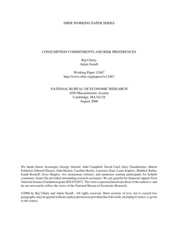
14For R 1 and Y 1, the equity premium is 5%/year, while the jump risk λ( implicit in option pricesis three times that of the true jump risk. Thus, the crash aversion parameter Y is roughly asimportant as relative risk aversion for the equity premium, but substantially more important for thecrash premium. Achieving the observed substantial disparity between λ( and λ using risk aversionalone ( Y ' 0) would require levels of R that most would find unpalatable, and which would implyan implausibly high equity premium.Since returns are i.i.d. under both the actual and risk-neutral distribution, the homogeneousagent model is not capable of capturing the dynamic anomalies discussed in section 1. The standardresults from regressing realized on implicit variance cannot be replicated here, because neither istime-varying in this model. Were there a time-varying volatility component in the dividend newsprocess, however, the difference between λ( and λ would affect the intercept from such regressionsbut could not explain why the slope estimate is less than 1. Second, the model cannot match the(observed tendency of λt to jump contemporaneously with substantial market drops. Finally, thei.i.d. return structure implies that implicit distributions should rapidly converge towardslognormality at longer maturities -- which does not accord with the maturity profile of the volatilitysmirk.Furthermore, Jackwerth’s (2000) anomaly cannot be replicated under homogeneous crashaversion. As discussed in Rosenberg and Engle (2000), Jackwerth’s implicit pricing kernel involvesthe projection of the actual pricing kernel upon asset payoffs. E.g., stock index options withterminal payoff V(St ) have an initial pricev0 'E0 [η t V(St )]η0' E0 V(St )E0[η t * St ](19)E0 [ηt ]/ E0 [V(St ) M(St ) ] ,where M(St ) has the usual properties of pricing kernels: it is nonnegative, and E0[ M(St ) ] ' 1 .It is shown in the appendix that for crash-averse preferences, this projection takes the form
15&RM(St ) ' κ(t) Stp St *λ e Y(20)p (St *λ )where κ(t) is a function of time and p (St * λ) is the probability density function of St conditionalupon a jump intensity of λ over (0, t). Implicit relative risk aversion is given by &M lnM(S) / M ln S .For Y ' 0 , one observes the strictly decreasing pricing kernel and constant relative risk aversionassociated with power utility. For Y 0 , it is proven in the appendix that ln M(St ) is a strictlydecreasing function of ln St that is illustrated below in Figure 3. Thus, this pricing kernel cannotreplicate the negative implicit risk aversion (positive slope) estimated by Jackwerth (2000) andRosenberg and Engle (2000) for some values of St . However, crash-averse preferences can replicatethe higher implicit risk aversion (steeper negative slope) for low ln St values that was estimated bythose authors and by Aït-Sahalia and Lo (2000).Jackwerth (2000, p.446) conjectures that the negative risk aversion estimate may beattributable to investors overestimating the crash risk relative to the observed ex post crashfrequency. Within this model, such overestimation is equivalent to a positive value of Y , and cannotgenerate the required divergences between objective and risk-neutral distributions. In equilibriumthe equity premium (15) is also positively affected by Y, shifting the mode of the objectiveln M(St)21.510.5ln(St / S0 )-0.3-0.2-0.10.10.20.3Figure 3. Log of the implicit pricing kernel conditional uponrealized returns. Calibration: t ' 1/12, σd ' .15, R ' Y ' 1,γd ' &.10, λ ' .25 .
16distribution sufficiently to the right to preclude observing Jackwerth’s anomaly. Of course, therecould still be an anomalous disparity between the risk-neutral distribution and the estimate of theobjective distribution.Jackwerth’s exploration of whether the divergence between the risk-neutral and estimatedobjective distributions is implausibly profitable is a separate issue. Within this framework, crashaversion can generate investment opportunities with high Sharpe ratios.For instance, theinstantaneous Sharpe ratio on writing crash insurance isλ( dt & Et [1*d N ' 1 ]Vart[1*d N ' 1]'(λ( & λ) dtλ dt (1 & λ dt)λ(& 1'λ(21)which can be substantially larger than the instantaneous Sharpe ratio µ / σ2 % λ k 2 on equity giveninvestors’ aversion to this type of risk. The put selling strategies examined in Jackwerth implicitlyinvolve a portfolio that is instantaneously long equity and short crash insurance. Since adding a highSharpe ratio investment to a market investment must raise instantaneous Sharpe ratios, this modelis consistent with the substantial profitability of option-writing strategies reported in Jackwe
tion of crash risk through option markets. A general equilibrium model is constructed in which relatively crash-tolerant option market makers insure crash-averse investors. Heterogeneity in attitudes towards crash risk is modeled via heter ogeneous state-dependent utility functions similar to those in Ho, Perraudin and Sørensen (1996).