WIXLIB

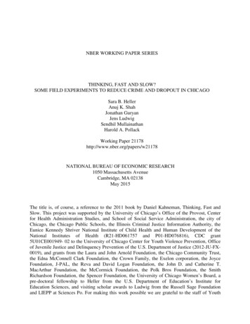
evidence for the model by examining how consumption adjustment patterns vary across goods.Section II develops the model and characterizes risk preferences. Section III presents applications,and Section IV concludes. All proofs are given in the appendix.I.MOTIVATING EVIDENCEWe begin by documenting some facts about consumption adjustment patterns at the householdlevel to motivate the model developed below.Table I shows expenditure shares for broad con-sumption categories such as housing and food using data from the Consumer Expenditure Survey.Our goal is to classify each of these categories as “commitment” or “adjustable,” in order to estimate the share of consumption that is xed over moderate-scale shocks. This estimate is useful incalibrating the model and gauging the extent to which commitments amplify risk aversion.2I.A.Frequency Classi cationA simple classi cation method is to de ne categories whose consumption is infrequently reducedas commitments.i from year tLet gcit denote the growth rate of consumption of category c by household1 to year t.Figure I plots histograms for the distribution of gcit for severalconsumption categories. We use food and housing data from the PSID (1968-1997), following theconventions established by Zeldes [1989] and Gruber [1997] in de ning these variables. The datafor the remaining categories is from the Consumer Expenditure Surveys (1990-1999). See the dataappendix for details on the data construction and de nitions.3For nondurable goods and services, gcit can be computed simply as the log change in reportedexpenditures from one year to the next. Figures 1a-1c show the resulting histograms for changesin nominal expenditure on food, entertainment, and health insurance.Measuring changes inconsumption of housing and other durable goods requires a di erent approach because the data donot give measures of the ‡ow consumption value of these goods. For housing, we rst determinewhether a household moved from year t1 to year t. If it did not, we de ne the change in housingconsumption as zero. For households that did move, we de ne the change in housing consumption2Calibrating the model requires a measure of the ‡ow consumption share of commitments rather than the expenditure shares reported in Table 1. While data on ‡ow consumption is unavailable for durables, aggregate expenditureshares in a representative sample are approximately equal to average consumption shares in a steady state economywith constant growth, depreciation, and interest rate. This fact allows us to interpret the shares in Table 1 as averageconsumption shares.3We use housing data from the PSID because the CEX drops movers. We use food data from the PSID forconsistency with the event-study analysis below (results from the CEX data are similar). Since the PSID gives dataon only food and housing consumption, we use CEX data to classify the remaining categories.4

as the log change in nominal rent for renters and the log change in the nominal market value ofthe houses for homeowners.4,5 We use an analogous approach in the CEX to de ne changes in carconsumption (see data appendix for details).For other durable goods, namely apparel and furniture/appliances, we do not have a measureof initial value of the durable stock in the data. For these categories, we analyze the level changein consumption instead of growth rate of consumption. We de ne the level change in consumptionas net expenditures (purchases minus sales) over a one year period in real 2000 dollars. Note thathouseholds can actively reduce their consumption of these durables (beyond natural decline due todepreciation) only by selling these durables in the secondary market, i.e. by having negative netexpenditures. Figure If shows the distribution of level changes in furniture consumption using thismethodology.Figure I indicates that food and entertainment are easily adjustable goods since their distributions are quite dispersed. In contrast, housing is infrequently adjusted, consistent with the largetransaction costs inherent in changing housing consumption (e.g., broker fees, monetary and utilitycosts of moving). Similarly, consumption of durable goods such as cars and furniture is infrequentlyadjusted, particularly downward, perhaps because market resale values are signi cantly lower thanactual values, creating an adjustment cost. Finally, the histogram for health insurance indicatesthat commitments extend beyond durables to services that involve contracts and penalties for earlytermination.6Figure I suggests a natural statistic for classifying categories into the “commitment” and “adjustable” bins – the fraction of households that report an active reduction in consumption.category whose consumption is di cult to cut is more of a commitment.ATable I reports thisstatistic for the consumption categories in the CEX, following the methodology illustrated in thehistograms. Using a cuto of 33 percent on the frequency of downward adjustments, the rst veconsumption categories fall into the “commitment”category, implying that commitments compriseapproximately 50 percent of the average household’s budget.4We use this methodology because ‡uctuations in rents or housing values due to asset price variation do notcorrespond to changes in housing consumption for non-movers. While this method misses changes in housingconsumption among non-movers due to remodelling, reductions in housing consumption through remodelling arepresumably infrequent.5For simplicity, we do not compute housing consumption growth rates for individuals who switch from owning torenting or vice versa (5.5 percent of observations). Since omitting these observations understates the frequency ofmoves, we adjust the fraction of zeros in the histogram (Figure 1b) to correct for this bias. See the data appendixfor details.6Late payments do not eliminate commitments. In the event of an income shock, the individual must still eventuallypay the bill. The ability to make late payments is simply an additional credit channel.5

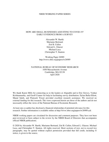
I.B.Wealth Shock Classi cationA limitation of the frequency classi cation method is that it does not shed light on how consumption is adjusted in response to shocks.Examining the response of consumption to wealthshocks is important because the key concept underlying our model is that some portions of thehousehold’s consumption bundle remain xed when moderate shocks occur.To provide such evidence, we conduct an event study analysis of unemployment shocks usingdata from the PSID spanning 1968 to 2003.In particular, we compare the food and housingconsumption responses of homeowners and renters to examine whether higher adjustment costs forhousing lead to less adjustment on that margin.We focus on heads of household between theages of 20 and 65 who report one unemployment spell during the panel. We construct event-studygraphs by normalizing the year of unemployment as 0 for all individuals, and de ning all otheryears relative to this base year (e.g., the year before the shock is -1, the year after the shock is 1). Observations with changes in the number of people in the household are excluded to avoidintroducing noise in the consumption measures because of changes in household composition.Figure IIa plots mean real annual growth rates of food and housing consumption, de ned asabove, for individuals who rented in year -1.7 In the year of job loss, food consumption falls fromits pre-unemployment level by 6.7 percent, while housing consumption falls by 4.3 percent. Thefraction of renters who move rises from 39.4 percent in year -1 to 45.3 percent in year 0. Renterswho do not move reduce food consumption by 5.7 percent on average, indicating that many rentersreduce food but not housing consumption in response to the shock. Figure IIb shows analogous gures for individuals who were homeowners in year -1. Homeowners reduce food consumption by9.1 percent in year 0, but reduce housing consumption by less than 0.1 percent on average. Thefraction of homeowners who move rises from 12.8 percent in year -1 to only 14.2 percent in year 0,indicating that homeowners’consumption bundles become more distorted in terms of food-housingcomposition than renters’bundles during unemployment spells.8 These ndings support the claimthat adjustment costs induce households to concentrate expenditure reductions on certain goodswhen moderate income shocks occur.The event studies suggest a second, more general de nition of “commitments”–categories that7These gures omit individuals who switch from owning to renting or vice versa. In Appendix C, we show thatincluding these switchers by computing the rental value of owning a house using Himmelberg et. al.’s [2005] user costof housing series does not a ect the results. Appendix C also gives summary statistics showing how homeowners andrenters in the PSID sample di er on observables, and shows that the event-study results are robust to controlling forthese observables and several other speci cation checks.8Note that the magnitude of the food consumption drop is not much larger for homeowners than renters. This ispresumably because homeowners are wealthier on average, and can therefore better smooth the shock intertemporally.6

are insensitive to moderate income shocks. Unfortunately, since the PSID contains data on onlyfood and housing, the e ect of unemployment shocks on consumption of other goods cannot beestimated. However, we expect that more goods would be classi ed as commitments under thiswealth-shock de nition than under the frequency of adjustment de nition used above. For example,while utility bills ‡uctuate over time as temperatures and energy costs change, it may be di cultto voluntarily change heating expenditures sharply in response to a shock if one does not move.Similarly, consumption of education and gasoline for vehicles may also be relatively unresponsiveto moderate shocks despite being volatile over time because of variation in input costs, lifecyclepatterns, etc. While utilities, fuel costs, and education do not involve explicit adjustment costs,they have a commitment-like property in that they may be di cult to adjust and force additionaladjustment on other margins. Hence, in our stylized two-good model, these categories a ect riskaversion in the same way as housing and other goods with adjustment costs. Including these goodsas “commitments” suggests an e ective commitment share closer to 65 percent.Irrespective of the details of the method used to de ne commitments, the key point is that asubstantial portion of consumption is in‡exible. The next section explores the implications of thisobservation for risk preferences.II.II.A.THEORYSetupConsider a household that lives for T periods and consumes two goods: adjustables, such as food(f ), and commitments, such as housing (x). Adjusting commitment consumption that provides xunits of services per period requires payment of an adjustment cost k x, where k 0.Thehousehold chooses a consumption path to maximize the expected value of lifetime utility:E0TXu(ft ; xt ),t 1where period utility u(f; x) is strictly increasing in both arguments, strictly concave, and threetimes continuously di erentiable. For simplicity, we assume that the household does not discountfuture utility and that the interest rate is zero.The household has a risky income stream denoted by yt . Let Wt denote wealth at the beginningof period t.The change in wealth, Wt 1Wt , is determined by income minus expenditure on7

current food and housing consumption, less moving costs kxt1in the event that the householddecides to move.9 The household’s dynamic budget constraint is(1)Wt 1 Wt yt 1ftxtkxt11fxt16 xt gfor 1tTtogether with the terminal condition WT 1 0. The timing of the household’s problem is asfollows. In period zero, the household selects a house x0 to maximize expected utility given initialwealth W0 and its knowledge of the distribution of the future path of income. The household beginsconsuming f and x in period 1, which it enters with wealth W1 W0 y1 and commitment x0 .In period 1 and all subsequent periods, consumption of ft and xt is chosen to maximize expectedutility, taking into account the cost of adjusting prior commitments.Note when choosing x0 in period 0, the household is aware of the commitment nature of thegood and takes into account its e ects on the welfare cost of shocks in subsequent periods. We focushere on characterizing consumption behavior and risk preferences in period 1, after the commitmentchoice has been made. From the perspective of period 1, x0 is a state variable that is e ectivelytreated as exogenous by the household. In this paper, we do not characterize the optimal policyfor x0 . Shore and Sinai [2005] explore this decision, and show that an increase in risk can eitherincrease or reduce x0 , depending on the distribution of the risk.We make two assumptions to simplify the analysis of the household’s problem. First, we abstractfrom capital market imperfections by allowing the household to borrow against future income.Second, we assume that all uncertainty in the economy is resolved in period 1: in particular, thehousehold learns the entire realization of fyt gTt 1 at the beginning of period 1. We discuss theimplications of relaxing these assumptions below.II.B.Consumption BehaviorThe optimal consumption policy in period 1 is governed by two state variables: prior commitPments x0 and lifetime wealth W W0 Tt 1 yt . Since the discount factor and interest rate arezero, and all uncertainty is resolved in period 1, the optimal consumption path is deterministic and‡at: ft f1 and xt x1 for all t 1; 2; :::; T . As a result, if the household ever moves, it moves inperiod 1.The decision to move in period 1 depends on a trade-o between the bene t of having the9While the consumption adjustment patterns documented above suggest that adjustment costs are larger forreductions than increases, we assume a symmetric adjustment cost for simplicity. Permitting asymmetric adjustmentcosts would not a ect the main qualitative results.8

optimal bundle of food and housing consumption and the transaction cost associated with reachingthat bundle. To characterize this decision formally, let v c (W; x0 ) denote the household’s valuefunction in period 1. Thenv c (W; x0 ) max v 0 (W; x0 ),v m (W; x0 )(2)where v 0 (W; x0 ) is maximized utility conditional on never moving, and v m (W; x0 ) is the maximizedutility of a household who moves in period 1. The optimal consumption choice of the householdhas a simple analytical solution if the utility function satis es the following conditions.A1 Limit properties of utility: limf !1 u1 (f; x) limx!1 u2 (f; x) 0; and limf !0 u(f; x) inf f 0 ;x0 u(f 0 ; x0 ) for all x.A2 The marginal utility of food is nondecreasing in housing consumption: u1;2 (f; x)0.Both of these conditions are satis ed for a wide class of utility functions, including (1) theconstant elasticity of substitution (CES) speci cation when the elasticity of substitution is notgreater than 1; and (2) separable power utility over the two goods as long as the coe cient ofrelative risk aversion for food is 1 or higher.Under these conditions, the agent’s consumptionpolicy in period 1 can be written as an (S,s) rule:Lemma 1. Under assumptions A1 and A2, for each x0 0 there exist s S such that(i) when W 2 (s; S), the optimal policy is not to move:xt x0andft W Tx0 :(ii) when W 2 (s; S), the optimal policy is to move, and(ft ; xt ) arg max fu(f; x) j f x (Wkx0 ) T g :(iii) when k increases, s falls and S increases.The intuition underlying this result is straightforward.a large negative wealth shock in period 1.Suppose that the agent experiencesThen he will be forced to reduce food consumptiondrastically in order to maintain the housing commitment that he previously made. Since such asharp reduction in food consumption causes a large reduction in utility, it becomes optimal to pay9

the adjustment cost and move into a smaller home. Conversely, if wealth rises sharply, rather thanallocating all of the extra wealth to food, whose marginal utility eventually diminishes to zero, itis preferable to pay the adjustment cost and upgrade to a large house.For smaller shocks, theutility gain from fully reoptimizing the consumption bundle is insu cient to o set the transactioncost, so there is an (S,s) band where the agent does not move.Assumptions A1 and A2 are useful in obtaining the (S,s) result because they guarantee thatthe agent moves for large shocks. A1 ensures that it is preferable to move to a smaller house thanto cut food consumption to zero. To understand the role of A2, consider the case where f and xare perfect substitutes. In that case, A2 is violated, and the household would never move, becausehousing and food are interchangeable. Note that these assumptions are su cient but not necessaryconditions for Lemma 1 and subsequent results. Empirical evidence shows that households follow(S,s) policies for goods that involve adjustment costs [Eberly 1994, Attanasio 2000, Martin 2003],suggesting that violations of assumptions A1 or A2, if any, are not large enough to cause deviationsfrom the intuitive (S,s) policy in practice.II.C.Risk PreferencesThe welfare cost of shocks, and thus the household’s risk preferences, are determined by theshape of the value function v c (W; x0 ) in period 1.We formally characterize this function in aseries of steps. Before proceeding, it is helpful to introduce some notation. Let v n (W ) denote thevalue function of a hypothetical agent who pays no adjustment costs for housing, and letn (W ) nnvWW W vW represent the period 1 coe cient of relative risk aversion (CRRA) over wealth forthis agent. Letc (W )represent the analogous parameter for an agent with commitments.10 Letf u11 f(f; x)u1denote the CRRA over food, and de ne"uf ;x u12 xu1as the elasticity of u1 (f; x) with respect to x. Note that bothfand "uf ;x are pure preferenceparameters: they depend on the level of f and x only, and not on the presence or absence ofadjustment costs.10Throughout, we use the convention that a superscript c refers to the presence of adjustment costs while asuperscript n refers to the case of no adjustment costs.10

Let f n (W ) and xn (W ) represent the optimal consumption choices in period 1 as a function oflifetime wealth W for a consumer who faces no adjustment costs. Let "nf;W denote the elasticityof food consumption with respect to wealth W in period 1 for this consumer and "cf;W the corresponding elasticity in the presence of adjustment costs. De ne the wealth elasticities of housing"nx;W and "cx;W analogously.E ect of commitments on CRRA. The CRRA over wealth in the benchmark case of a consumerwho faces no adjustment costs isn(W ) (3) nvWWW nvWnf "f;WW@f@xu11 @W u12 @Wu1"uf ;x "nx;W .The intuition for this expression is as follows. By the envelope theor

Raj Chetty and Adam Szeidl NBER Working Paper No. 12467 August 2006 JEL No. E2, H2, H5, J21, J64 ABSTRACT Many households devote a large fraction of their budgets to "consumption commitments" -- goods that involve transaction costs and are infrequently adjusted. This paper characterizes risk preferences in an expected utility model with .