Transcription
Three tutorial lectures on entropy and counting1David Galvin21st Lake Michigan Workshop on Combinatoricsand Graph Theory, March 15–16 20141 Thesenotes were prepared to accompany a series of tutorial lectures given by the author atthe 1st Lake Michigan Workshop on Combinatorics and Graph Theory, held at Western MichiganUniversity on March 15–16 2014.2 dgalvin1@nd.edu; Department of Mathematics, University of Notre Dame, Notre Dame IN46556. Supported in part by National Security Agency grant H98230-13-1-0248.
AbstractWe explain the notion of the entropy of a discrete random variable, and derive some of its basic properties. We then show through examples how entropy can be useful as a combinatorialenumeration tool. We end with a few open questions.
Contents1 Introduction2 The2.12.22.32.42.52.62.72.82.91basic notions of entropyDefinition of entropy . . . . . . . . . . . . . . . . . . . . . . . . . . . . .Binary entropy . . . . . . . . . . . . . . . . . . . . . . . . . . . . . . . .The connection between entropy and counting . . . . . . . . . . . . . . .Subadditivity . . . . . . . . . . . . . . . . . . . . . . . . . . . . . . . . .Shearer’s lemma . . . . . . . . . . . . . . . . . . . . . . . . . . . . . . . .Hiding the entropy in Shearer’s lemma . . . . . . . . . . . . . . . . . . .Conditional entropy . . . . . . . . . . . . . . . . . . . . . . . . . . . . . .Proofs of Subadditivity (Property 2.7) and Shearer’s lemma (Lemma 2.8)Conditional versions of the basic properties . . . . . . . . . . . . . . . . .2244556789.10101112134 Embedding copies of one graph in another4.1 Introduction to the problem . . . . . . . . . . . . . . . . . . . . . . . . . . .4.2 Background on fractional covering and independent sets . . . . . . . . . . . .4.3 Proofs of Theorem 4.1 and 4.2 . . . . . . . . . . . . . . . . . . . . . . . . . .141415165 Brégman’s theorem (the Minc conjecture)5.1 Introduction to the problem . . . . . . . . . . . . . . . . . . . . . . . . . . .5.2 Radhakrishnan’s proof of Brégman’s theorem . . . . . . . . . . . . . . . . . .5.3 Alon and Friedland’s proof of the Kahn-Lovász theorem . . . . . . . . . . . .171718206 Counting proper colorings of a regular graph6.1 Introduction to the problem . . . . . . . . . . . . . . . . . . . . . . . . . . .6.2 A tight bound in the bipartite case . . . . . . . . . . . . . . . . . . . . . . .6.3 A weaker bound in the general case . . . . . . . . . . . . . . . . . . . . . . .212124257 Open problems7.1 Counting matchings . . . . . . . . . . . . . . . . . . . . . . . . . . . . . . . .7.2 Counting homomorphisms . . . . . . . . . . . . . . . . . . . . . . . . . . . .2626278 Bibliography of applications of entropy to combinatorics283 Four quick applications3.1 Sums of binomial coefficients .3.2 The coin-weighing problem . .3.3 The Loomis-Whitney theorem3.4 Intersecting families . . . . . .1.IntroductionOne of the concerns of information theory is the efficient encoding of complicated sets bysimpler ones (for example, encoding all possible messages that might be sent along a channel,1
by as small as possible a collection of 0-1 vectors). Since encoding requires injecting thecomplicated set into the simpler one, and efficiency demands that the injection be closeto a bijection, it is hardly surprising that ideas from information theory can be useful incombinatorial enumeration problems.These notes, which were prepared to accompany a series of tutorial lectures given at the1st Lake Michigan Workshop on Combinatorics and Graph Theory, aim to introduce theinformation-theoretic notion of the entropy of a discrete random variable, derive its basicproperties, and show how it can be used as a tool for estimating the size of combinatoriallydefined sets.The entropy of a random variable is essentially a measure of its degree of randomness,and was introduced by Claude Shannon in 1948. The key property of Shannon’s entropythat makes it useful as an enumeration tool is that over all random variables that take onat most n values with positive probability, the ones with the largest entropy are those whichare uniform on their ranges, and these random variables have entropy exactly log2 n. So ifC is a set, and X is a uniformly randomly selected element of C, then anything that can besaid about the entropy of X immediately translates into something about C . Exploitingthis idea to estimate sizes of sets goes back at least to a 1963 paper of Erdős and Rényi [21],and there has been an explosion of results in the last decade or so (see Section 8).In some cases, entropy provides a short route to an already known result. This is the casewith three of our quick examples from Section 3, and also with two of our major examples,Radhakrishnan’s proof of Brégman’s theorem on the maximum permanent of a 0-1 matrixwith fixed row sums (Section 5), and Friedgut and Kahn’s determination of the maximumnumber of copies of a fixed graph that can appear in another graph on a fixed number ofedges (Section 4). But entropy has also been successfully used to obtain new results. Thisis the case with one of our quick examples from Section 3, and also with the last of ourmajor examples, Galvin and Tetali’s tight upper bound of the number of homomorphisms toa fixed graph admitted by a regular bipartite graph (Section 6, generalizing an earlier specialcase, independent sets, proved using entropy by Kahn). Only recently has a non-entropyapproach for this latter example been found.In Section 2 we define, motivate and derive the basic properties of entropy. Section3 presents four quick applications, while three more substantial applications are given inSections 4, 5 and 6. Section 7 presents some open questions that are of particular interestto the author, and Section 8 gives a brief bibliographic survey of some of the uses of entropyin combinatorics.The author learned of many of the examples that will be presented from the lovely 2003survey paper by Radhakrishnan [50].22.1The basic notions of entropyDefinition of entropyThroughout, X, Y , Z etc. will be discrete random variables (actually, random variablestaking only finitely many values), always considered relative to the same probability space.We write p(x) for Pr({X x}). For any event E we write p(x E) for Pr({X x} E), and2
we write p(x y) for Pr({X x} {Y y}).Definition 2.1. The entropy H(X) of X is given byXH(X) p(x) log p(x),xwhere x varies over the range of X.Here and everywhere we adopt the convention that 0 log 0 0, and that the logarithmis always base 2.Entropy was introduced by Claude Shannon in 1948 [56], as a measure of the expectedamount of information contained in a realization of X. It is somewhat analogous to thenotion of entropy from thermodynamics and statistical physics, but there is no perfect correspondence between the two notions. (Legend has it that the name “entropy” was applied toShannon’s notion by von Neumann, who was inspired by the similarity to physical entropy.The following recollection of Shannon was reported in [58]: “My greatest concern was whatto call it. I thought of calling it ‘information’, but the word was overly used, so I decidedto call it ‘uncertainty’. When I discussed it with John von Neumann, he had a better idea.Von Neumann told me, ‘You should call it entropy, for two reasons. In the first place youruncertainty function has been used in statistical mechanics under that name, so it alreadyhas a name. In the second place, and more important, nobody knows what entropy reallyis, so in a debate you will always have the advantage’.”)In the present context, it is most helpful to (informally) think of entropy as a measureof the expected amount of surprise evinced by a realization of X, or as a measure of thedegree of randomness of X. A motivation for this way of thinking is the following: let S be afunction that measures the surprise evinced by observing an event occurring in a probabilityspace. It’s reasonable to assume that the surprise associated with an event depends only onthe probability of the event, so that S : [0, 1] R (with S(p) being the surprise associatedwith seeing an event that occurs with probability p).There are a number of conditions that we might reasonably impose on S:1. S(1) 0 (there is no surprise on seeing a certain event);2. If p q, then S(p) S(q) (rarer events are more surprising);3. S varies continuously with p;4. S(pq) S(p) S(q) (to motivate this imposition, consider two independent eventsE and F with Pr(E) p and Pr(F ) q. The surprise on seeing E F (which isS(pq)) might reasonable be taken to be the surprise on seeing E (which is S(p)) plusthe remaining surprise on seeing F , given that E has been seen (which should be S(q),since E and F are independent); and5. S(1/2) 1 (a normalizing condition).Proposition 2.2. The unique function S that satisfies conditions 1 through 5 above is S(p) log p3
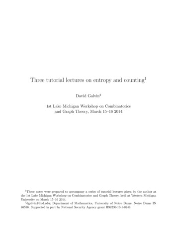
The author first saw this proposition in Ross’s undergraduate textbook [53], but it isundoubtedly older than this.Exercise 2.3. Prove Proposition 2.2 (this is relatively straightforward).Proposition 2.2 says that H(X) does indeed measure the expected amount of surpriseevinced by a realization of X.2.2Binary entropyWe will also use “H(·)” as notation for a certain function of a single real variable, closelyrelated to entropy.Definition 2.4. The binary entropy function is the function H : [0, 1] R given byH(p) p log p (1 p) log(1 p).Equivalently, H(p) is the entropy of a two-valued (Bernoulli) random variable that takes itstwo values with probability p and 1 p.The graph of H(p) is shown above (x-axis is p). Notice that it has a unique maximum atp 1/2 (where it takes the value 1), rises monotonically from 0 to 1 as p goes from 0 to 1/2,and falls monotonically back to 0 as p goes from 1/2 to 1. This reflects that idea that thereis no randomness in the flip of a two-headed or two-tailed coin (p 0, 1), and that amongbiased coins that come up heads with probability p, 0 p 1, the fair (p 1/2) coin is insome sense the most random.2.3The connection between entropy and countingTo see the basic connection between entropy and counting, we need Jensen’s inequality.Theorem 2.5. Let f : [a, b] R be a continuous, concave function, and let p1 , . . . , pn benon-negative reals that sum to 1. For any x1 , . . . , xn [a, b],!nnXXpi f (xi ) fp i xi .i 1i 14
Noting that the logarithm function is concave, we have the following corollary, the firstbasic property of entropy.Property 2.6. (Maximality of the uniform) For random variable X,H(X) log range(X) where range(X) is the set of values that X takes on with positive probability. If X isuniform on its range (taking on each value with probability 1/ range(X) ) then H(X) log range(X) .This property of entropy makes clear why it can be used as an enumeration tool. SupposeC is some set whose size we want to estimate. If X is a random variable that selects an elementfrom C uniformly at random, then C 2H(X) , and so anything that can be said about H(X)translates directly into something about C .2.4SubadditivityIn order to say anything sensible about H(X), and so make entropy a useful enumerationtool, we need to derive some further properties. We begin with subadditivity. A vector(X1 , . . . , Xn ) of random variables is itself a random variable, and so we may speak sensiblyof H(X1 , . . . , Xn ). Subadditivity relates H(X1 , . . . , Xn ) to H(X1 ), H(X2 ), etc.Property 2.7. (Subadditivity) For random vector (X1 , . . . , Xn ),H(X1 , . . . , Xn ) nXH(Xi ).i 1Given the interpretation of entropy as expected surprise, Subadditivity is reasonable:considering the components separately cannot cause less surprise to be evinced than considering them together, since any dependence among the components will only reduce surprise.We won’t prove Subadditivity now, but we will derive it later (Section 2.8) from a combination of other properties. Subadditivity is all that is needed for our first two applicationsof entropy, to estimating the sum of binomial coefficients (Section 3.1), and (historicallythe first application of entropy) to obtaining a lower bound for the coin-weighing problem(Section 3.2).2.5Shearer’s lemmaSubadditivity was significantly generalized in Chung et al. [12] to what is known as Shearer’slemma. Here and throughout we use [n] for {1, . . . , n}.Lemma 2.8. (Shearer’s lemma) Let F be a family of subsets of [n] (possibly with repeats)with each i [n] included in at least t members of F. For random vector (X1 , . . . , Xn ),1XH(XF ),H(X1 , . . . , Xn ) t F Fwhere XF is the vector (Xi : i F ).5
To recover Subadditivity from Shearer’s lemma, take F to be the family of singletonsubsets of [n]. The special case where F {[n] \ i : i [n]} is Han’s inequality [31].We’ll prove Shearer’s lemma in Section 2.8. A nice application to bounding the volume ofa body in terms of the volumes of its co-dimension 1 projections is given in Section 3.3, anda more substantial application, to estimating the maximum number of copies of one graphthat can appear in another, is given in Section 4.2.6Hiding the entropy in Shearer’s lemmaLemma 2.8 does not appear in [12] as we have stated it; the entropy version can be read outof the proof from [12] of the following purely combinatorial version of the lemma. For a setof subsets A of some ground-set U , and a subset F of U , the trace of A on F istraceF (A) {A F : A A};that is, traceF (A) is the set of possible intersections of elements of A with F .Lemma 2.9. (Combinatorial Shearer’s lemma) Let F be a family of subsets of [n] (possiblywith repeats) with each i [n] included in at least t members of F. Let A be another set ofsubsets of [n]. ThenY1 A traceF (A) t .F FProof. Let X be an element of A chosen uniformly at random. View X as the random vector(X1 , . . . , Xn ), with Xi the indicator function of the event {i X}. For each F F we have,using Maximality of the uniform (Property 2.6),H(XF ) log traceF (A) ,as so applying Shearer’s lemma with covering family F we getH(X) 1Xlog traceF (A) .t F FUsing H(X) log A (again by Maximality of the uniform) and exponentiating, we get theclaimed bound on A .This proof nicely illustrates the general idea underlying every application of Shearer’slemma: a global problem (understanding H(X1 , . . . , Xn )) is reduced to a collection of localones (understanding H(XF ) for each F ), and these local problems can be approached usingvarious properties of entropy.Some applications of Shearer’s lemma in its entropy form could equally well be presentedin the purely combinatorial setting of Lemma 2.9; an example is given in Section 3.4, wherewe use Combinatorial Shearer’s lemma to estimate the size of the largest family of graphs onn vertices any pair of which have a triangle in common. More complex examples, however,such as those presented in Section 6, cannot be framed combinatorially, as they rely on theinherently probabilistic notion of conditioning.6
2.7Conditional entropyMuch of the power of entropy comes from being able to understand the relationship betweenthe entropies of dependent random variables. If E is any event, we define the entropy of Xgiven E to beXH(X E) p(x E) log p(x E),xand for a pair of random variables X, Y we define the entropy of X given Y to beXXH(X Y ) EY (H(X {Y y})) p(y)p(x y) log p(x y).yxThe basic identity related to conditional entropy is the chain rule, that pins down how theentropy of a random vector can be understood by revealing the components of the vectorone-by-one.Property 2.10. (Chain rule) For random variables X and Y ,H(X, Y ) H(X) H(Y X).More generally,H(X1 , . . . , Xn ) nXH(Xi X1 , . . . , Xi 1 ).i 1Proof. We just prove the first statement, with the second following by induction. For thefirst,XX p(x) log p(x) p(x, y) log p(x, y) H(X, Y ) H(X) xx,y Xp(x)XXp(x)X p(y x) log p(x)p(y x) p(x) log p(x)Xp(x)xyxXxyx p(y x) log p(x)p(y x) Xp(y x) log p(x)y! Xp(x)XxyXX p(y x) log p(x)p(y x) p(y x) log p(x)! p(x)x p(y x) log p(y x)y H(X Y ).The key point is in the third equality: for each fixed x,Pyp(y x) 1.Another basic property related to conditional entropy is that increasing conditioningcannot increase entropy. This makes intuitive sense — the surprise evinced on observing Xshould not increase if we learn something about it through an observation of Y .7
Property 2.11. (Dropping conditioning) For random variables X and Y ,H(X Y ) H(X).Also, for random variable ZH(X Y, Z) H(X Y ).Proof. We just prove the first statement, with the proof ofPthe second being almost identical.For the first, we again use the fact that for each fixed x, y p(y x) 1, which will allow usto apply Jensen’s inequality in the inequality below. We also use p(y)p(x y) p(x)p(y x)repeatedly. We haveXXH(X Y ) p(y) p(x y) log p(x y) yxXXp(x)x X p(y x) log p(x y)yp(x) logX p(y x)!p(x y)!XX p(y) p(x) logp(x)xyX p(x) log p(x)xyx H(X).2.8Proofs of Subadditivity (Property 2.7) and Shearer’s lemma(Lemma 2.8)The subadditivity of entropy follows immediately from a combination of the Chain rule(Property 2.10) and Dropping conditioning (Property 2.11).The original proof of Shearer’s lemma from [12] involved an intricate and clever induction.Radhakrishnan and Llewellyn (reported in [50]) gave the following lovely proof using theChain rule and Dropping conditioning.Write F F as F {i1 , . . . , ik } with i1 i2 . . . ik . We haveH(XF ) H(Xi1 , . . . , Xik )kX H(Xij (Xi : j))j 1 kXH(Xij X1 , . . . , Xij 1 ).j 18
The inequality here is an application of Dropping conditioning. If we sum this last expressionover all F F, then for each i [n] the term H(Xi X1 , . . . , Xi 1 ) appears at least t timesand soXH(XF ) tF FnXH(Xi X1 , . . . , Xi 1 )i 1 tH(X),the equality using the Chain rule. Dividing through by t we obtain Shearer’s lemma.2.9Conditional versions of the basic propertiesConditional versions of each of Maximality of the uniform, the Chain rule, Subadditivity,and Shearer’s lemma are easily proven, and we merely state the results here.Property 2.12. (Conditional maximality of the uniform) For random variable X and eventE,H(X E) log range(X E) where range(X E) is the set of values that X takes on with positive probability, given that Ehas occurred.Property 2.13. (Conditional chain rule) For random variables X, Y and Z,H(X, Y Z) H(X Z) H(Y X, Z).More generally,H(X1 , . . . , Xn Z) nXH(Xi X1 , . . . , Xi 1 , Z).i 1Property 2.14. (Conditional subadditivity) For random vector (X1 , . . . , Xn ), and randomvariable Z,nXH(X1 , . . . , Xn Z) H(Xi Z).i 1Lemma 2.15. (First conditional Shearer’s lemma) Let F be a family of subsets of [n] (possibly with repeats) with each i [n] included in at least t members of F. For random vector(X1 , . . . , Xn ) and random variable Z,H(X1 , . . . , Xn Z) 1XH(XF Z).t F FA rather more powerful and useful conditional version of Shearer’s lemma, that may beproved exactly as we proved Lemma 2.8, was given by Kahn [36].9
Lemma 2.16. (Second conditional Shearer’s lemma) Let F be a family of subsets of [n](possibly with repeats) with each i [n] is included in at least t members of F. Let be apartial order on [n], and for F F say that i F if i x for each x F . For randomvector (X1 , . . . , Xn ),H(X1 , . . . , Xn ) 1XH(XF {Xi : i F }).t F FExercise 2.17. Give proofs of all the properties and lemmas from this section.3Four quick applicationsHere we give four fairly quick applications of the entropy method in combinatorial enumeration.3.1Sums of binomial coefficientsThere is clearly a connection between entropy and the binomial coefficients; for example,nStirling’s approximation to n! (n! (n/e) 2πn as n ) gives n2H(α)n p(1)αn2πnα(1 α)for any fixed 0 α 1. Here is a nice bound on the sum of all the binomial coefficientsup to αn, that in light of (1) is relatively tight, and whose proof nicely illustrates the use ofentropy.Theorem 3.1. Fix α 1/2. For all n,X n i αni 2H(α)n . PProof. Let C be the set of all subsets of [n] of size at most αn; note that C i αn ni .Let X be a uniformly chosen member of C; by Maximality of the uniform, it is enough toshow H(X) H(α)n.View X as the random vector (X1 , . . . , Xn ), where Xi is the indicator function of theevent {i X}. By Subadditivity and symmetry,H(X) H(X1 ) . . . H(Xn ) nH(X1 ).So now it is enough to show H(X1 ) H(α). To see that this is true, note that H(X1 ) H(p), where p Pr(1 X). We have p α (conditioned on X having size αn, Pr(i X)is exactly α, and conditioned on X having any other size it is strictly less than α), and so,since α 1/2, H(p) H(α).Theorem 3.1 can be used to quickly obtain the following concentration inequality for thebalanced (p 1/2) binomial distribution, a weak form of the Chernoff bound.10
Exercise 3.2. Let X be a binomial random variable with parameters n and 1/2. Show thatfor every c 0,2Pr( X n/2 cσ) 21 c /2 , where σ n/2 is the standard deviation of X.3.2The coin-weighing problemSuppose we are given n coins, some of which are pure and weigh a grams, and some of whichare counterfeit and weight b grams, with b a. We are given access to an accurate scale (nota balance), and wish to determine which are the counterfeit coins using as few weighingsas possible, with a sequence of weighings announced in advance. How many weighings areneeded to isolate the counterfeit coins? (A very specific version of this problem is due toShapiro [57].)When a set of coins is weighed, the information obtained is the number of counterfeitcoins among that set. Suppose that we index the coins by elements of [n]. If the sequenceof subsets of coins that we weigh is D1 , . . . , D , then the set D {D1 , . . . , D } must formwhat is called a distinguishing family for [n] — it must be such that for every A, B [n]with A 6 B, there is a Di D with A Di 6 B Di — for if not, and the Di ’sfail to distinguish a particular pair A, B, then our weighings would not be able distinguishbetween A or B being the set of counterfeit coins. On the other hand, if the Di do forma distinguishing family, then they also form a good collection of weighings — if A is thecollection of counterfeit coins, then on observing the vector ( A Di : i 1, . . . , ) we candetermine A, since A is the unique subset of [n] that gives rise to that particular vector ofintersections.It follows that determining the minimum number of weighings required is equivalent tothe combinatorial question of determining f (n), the minimum size of a distinguishing familyfor [n]. Cantor and Mills [10] and Lindström [40] independently established the upper bound log log n2n1 Of (n) log nlog nwhile Erdős and Rényi [21] and (independently) Moser [47] obtained the lower bound 12nf (n) 1 Ω.log nlog n(2)(See the note at the end of [21] for the rather involved history of these bounds). Here we givea short entropy proof of (2). A proof via information theory of a result a factor of 2 weakerwas described (informally) by Erdős and Rényi [21]; to the best of our knowledge this is thefirst application of ideas from information theory to a combinatorial problem. Pippinger [48]recovered the factor of 2 via a more careful entropy argument.Let X be a uniformly chosen subset of [n], so that (by Maximality of the uniform)H(X) n. By the discussion earlier, observing X is equivalent to observing the vector( X Di : i 1, . . . , ) (both random variables have the same distribution), and soH(X) H(( X Di : i 1, . . . , )) Xi 111H( X Di ),
the inequality by Subadditivity. Since X Di can take on at most n 1 values, we have(again by Maximality of the uniform) H( X Di ) log(n 1). Putting all this togetherwe obtain (as Erdős and Rényi did)n H(X) log(n 1)or n/ log(n 1), which falls short of (2) by a factor of 2.To gain back this factor of 2, we need to be more careful in estimating H( X Di ).Observe that X Di is a binomial random variable with parameters di and 1/2, wheredi Di , and so has entropy!di Xdi j2di .2 logdijjj 0If we can show that this is at most (1/2) log di C (where C is some absolute constant),then the argument above gives 1log n O(1) ,n 2which implies (2). We leave the estimation of the binomial random variable’s entropy asan exercise; the intuition is that the vast majority of the mass of the binomial is within10 (say) standard deviations of the mean (a consequence, for example, of Exercise 3.2, butTchebychev’s inequality would work fine here), and so only di of the possible values thatthe binomial takes on contribute significantly to its entropy.Exercise 3.3. Show that there’s a constant C 0 such that for all m,!m Xlog mm j2m C.2 logm2jjj 03.3The Loomis-Whitney theoremHow large can a measurable body in Rn be, in terms of the volumes of its (n 1)-dimensionalprojections? The following theorem of Loomis and Whitney [43] gives a tight bound. Fora measurable body B in Rn , and for each j [n], let Bj be the projection of B onto thehyperplane xj 0; that is, Bj is the set of all (x1 , . . . , xj 1 , xj 1 , . . . , xn ) such that there issome xj R with (x1 , . . . , xj 1 , xj , xj 1 , . . . , xn ) B.Theorem 3.4. Let B be a measurable body in Rn . Writing · for volume, B nY Bj 1/(n 1) .j 1This bound is tight, for example when B is a cube.12
Proof. We prove the result in the case when B is a union of axis-parallel cubes with sidelengths 1 centered at points with integer coordinates (and we identify a cube with thecoordinates of its center); the general result follows from standard scaling and limiting arguments.Let X be a uniformly selected cube from B; we write X as (X1 , . . . , Xn ), where Xi is theith coordinate of the cube. We upper bound H(X) by applying Shearer’s lemma (Lemma2.8) with F {F1 , . . . , Fn }, where Fj [n] \ j. For this choice of F we have t n 1. Thesupport of XFj (i.e., the set of values taken by XFj with positive probability) is exactly (theset of centers of the (d 1)-dimensional cubes comprising) Bj . So, using Maximality of theuniform twice, we havelog B H(X)n1 XH(XFj ) n 1 j 1n 1 Xlog Bj ,n 1 j 1from which the theorem follows.3.4Intersecting familiesLet G be a family of graphs on vertex set [n], with the property that for each G1 , G2 G,G1 G2 contains a triangle (i.e, there are three vertices i, j, k such that each of ij, ik, jk isin the edge set of both G1 and G2 ). At most how large can G be? This question was firstraised by Simonovits and Sós in 1976.nCertainly G can be as large as 2( 2 ) 3 : consider the family G of all graphs that includena particular triangle. In the other direction, it can’t be larger than 2( 2 ) 1 , by virtue of thewell-known result that a family of distinct sets on ground set of size m, with the propertythat any two members of the family have non-empty intersection, can have cardinality atnm 1most 2(the edge sets of elements of G certainly form such a family, with m 2 ). In[12] Shearer’s lemma is used to improve this easy upper bound.nTheorem 3.5. With G as above, G 2( 2 ) 2 .Proof. Identify each graph G G with its edge set, so that G is now a set of subsetsof a ground-set U of size n2 . For each unordered equipartition A B [n] (satisfying A B 1), let U (A, B) be the subset of U consisting of all those edges that lie entirelyinside A or entirely inside B. We will apply Combinatorial Shearer’s lemma with F {U (A, B)}.Let m U (A, B) (this is independent of the particular choice of equipartition). Notethat n/2 2 2 if n is evenm bn/2cdn/2e 2if n is odd;213
in either case, m 1 n2 2 . Note also that by a simple double-counting argument we have nm F t(3)2where t is the number of elements of F in which each element of U occurs.Observe that traceU (A,B) (G) forms an intersecting family of subsets of U (A, B); indeed,for any G, G0 G, G G0 has a triangle T , and since the complement of U (A, B) (in U ) istriangle-free (viewed as a graph on [n]), at least one of the edges of T must meet U (A, B).So, traceU (A,B) (G) 2m 1 .By Lemma 2.9, F 2m 1 tn1 2( 2 )(1 m )n 2( 2 ) 2 , G as claimed (the equality here uses (3)).Recently Ellis, Filmus and Friedgut [18] used discrete Fourier analysis to obtain the sharpnbound G 2( 2 ) 3 that had been conjectured by Simonovits and Sós.4Embedding copies of one graph in anotherWe now move on to our first more substantial application of entropy to combinatorial enumeration; the problem of maximizing the number of copies of a graph that can be embeddedin a graph on a fixed number of edges.4.1Introduction to the problemAt most how many copies of a fixed graph H can there be in a graph with edges? More formally, define an embedding of a graph H into a graph G as an injective function f from V (H)to V (G) with the property that f (x)f (y) E(G) whenever xy E(H). Let embed(H, G) bethe number of embeddings of H into G, and let embed(H, ) be the maximum of embed(H, G)as G varies over all graphs on edges. The question we are asking is: what is the value ofembed(H, ) for each H and ?Consider for example H K3 , the triangle. Fix G with edges. Suppose that x V (H)is mapped to v V (G). At most how many ways can this partial embedding be completed?Certainly no more that 2 ways (the remaining two vertices of H must be mapped, in anordered way, to one of the edges of G); but also, no more than dv (dv 1) d2v ways, wheredv is the degree of v (the remaining two verticesof H must be mapped, in an ordered way, 2to neighbors of v). Since min{dv , 2 } dv 2 , a simple union bound givesX embed(H, G) dv 2 2 2 3/2 ,v V (G)14
and so embed(H,
1These notes were prepared to accompany a series of tutorial lectures given by the author at the 1st Lake Michigan Workshop on Combinatorics and Graph Theory, held at Western Michigan University on March 15{16 2014. 2dgalvin1@nd.edu; Department of Mathematics, University of Notre Dame, Notre Dame IN 46556.