Transcription
NBER WORKING PAPER SERIESFACTOR MOMENTUM AND THE MOMENTUM FACTORSina EhsaniJuhani T. LinnainmaaWorking Paper 25551http://www.nber.org/papers/w25551NATIONAL BUREAU OF ECONOMIC RESEARCH1050 Massachusetts AvenueCambridge, MA 02138February 2019We thank Ing-Haw Cheng, John Cochrane, Mark Grinblatt, Jon Lewellen, Paulo Maio(discussant), Sheridan Titman, Ivo Welch, and Guofu Zhou for valuable comments. We aregrateful for the feedback by the conference and seminar participants at the Mark GrinblattRetirement Conference at UCLA, Washington University in St. Louis, DePaul University, BaruchCollege, University of Texas - Rio Grande Valley, Clemson University, Northern IllinoisUniversity, and the 2018 Midwest Finance Association. Linnainmaa is affiliated with Citadel andResearch Affiliates. Neither Citadel nor Research Affiliates provided any funding for thisresearch. The views expressed herein are those of the authors and do not necessarily reflect theviews of the National Bureau of Economic Research.NBER working papers are circulated for discussion and comment purposes. They have not beenpeer-reviewed or been subject to the review by the NBER Board of Directors that accompaniesofficial NBER publications. 2019 by Sina Ehsani and Juhani T. Linnainmaa. All rights reserved. Short sections of text, notto exceed two paragraphs, may be quoted without explicit permission provided that full credit,including notice, is given to the source.
Factor Momentum and the Momentum FactorSina Ehsani and Juhani T. LinnainmaaNBER Working Paper No. 25551February 2019JEL No. G11,G12,G40ABSTRACTMomentum in individual stock returns emanates from momentum in factor returns. Most factorsare positively autocorrelated: the average factor earns a monthly return of 1 basis point followinga year of losses and 53 basis points following a positive year. Factor momentum explains allforms of individual stock momentum. Stock momentum strategies indirectly time factors: theyprofit when the factors remain autocorrelated, and crash when these autocorrelations break down.Our key result is that momentum is not a distinct risk factor; it aggregates the autocorrelationsfound in all other factors.Sina EhsaniGraham School of ManagementSaint Xavier University3825 W 103rd StChicago, IL 60655United Statesehsani@sxu.eduJuhani T. LinnainmaaUniversity of Southern CaliforniaMarshall School of Business701 Exposition Blvd, Ste. 231Los Angeles, CA 90089-1422and NBERjuhani.linnainmaa@marshall.usc.edu
1IntroductionMomentum appears to violate the efficient market hypothesis in its weakest form. Past returnsshould not predict future returns if asset prices respond to new information immediately and tothe right extent—unless past returns correlate with changes in systematic risk. Researchers havesought to explain the profitability of momentum strategies with time-varying risk, behavioral biases,and trading frictions.1 At the same time, the pervasiveness of momentum over time and acrossasset classes has given momentum the status of an independent factor: models without momentumcannot explain it and those with momentum cannot explain anything more than just momentum(Fama and French, 2016).2 In this paper we show that momentum is not a distinct risk factor:it aggregates the autocorrelations found in all other factors. Rather than being unrelated to theother factors, momentum in fact relates to all of them.We first show that factors’ prior returns are informative about their future returns. Smallstocks, for example, are likely to outperform big stocks when they have done so over the prior year.This effect is economically and statistically large among the 20 factors we study: The average factorearns 52 basis points per month following a year of gains but just 2 basis points following a yearof losses. The difference in these average returns is significant with a t-value of 4.67. This resultis not specific to the use of obscure asset pricing factors: we work with the major factors that areregularly updated and published by academics and a hedge fund.A time-series factor momentum strategy is a strategy that bets on this continuation in factor1See, for example, Conrad and Kaul (1998), Berk et al. (1999), Johnson (2002), and Sagi and Seasholes (2007)for risk-based explanations; Daniel et al. (1998), Hong and Stein (1999), Frazzini et al. (2012), Cooper et al. (2004),Griffin et al. (2003), and Asness et al. (2013) for behavioral explanations; and Korajczyk and Sadka (2004), Lesmondet al. (2004), and Avramov et al. (2013) for trading friction-based explanations.2Jegadeesh (1990) and Jegadeesh and Titman (1993) document momentum in the cross section of stocks, Jostovaet al. (2013) in corporate bonds, Beyhaghi and Ehsani (2017) in corporate loans, Hendricks et al. (1993), Brownand Goetzmann (1995), Grinblatt et al. (1995), and Carhart (1997) in mutual funds, Baquero et al. (2005), Boyson(2008), and Jagannathan et al. (2010) in hedge funds, Bhojraj and Swaminathan (2006), Asness et al. (2013), andMoskowitz et al. (2012) in major futures contracts, Miffre and Rallis (2007) and Szakmary et al. (2010) in commodityfutures, Menkhoff et al. (2012) in currencies, and Lee et al. (2014) in credit default swaps.1
Figure 1: Individual stock momentum versus factor momentum.This figure shows tvalues associated with alphas for five momentum strategies that trade individual stocks and afactor momentum strategy that trades 20 factors. For individual stock momentum strategies, wereport t-values from the five-factor model (yellow bars) and this model augmented with factormomentum (blue bars). For the factor momentum strategy, we report t-values from the five-factormodel (yellow bar) and this model augmented with all five individual stock momentum strategies(blue bar). The dashed line denotes a t-value of 1.96.returns. It is long the factors with positive returns and short those with negative returns. Thistime-series momentum strategy earns an annualized return of 4.2% (t-value 7.04). We showthat this strategy dominates the cross-sectional strategy because it is a pure bet on the positiveautocorrelations in factor returns. A cross-sectional strategy, by contrast, also bets that a highreturn on a factor predicts low returns on the other factors (Lo and MacKinlay, 1990); in the data,however, high return on any factor predicts high returns on all factors.3Momentum in factor returns transmits into the cross section of security returns, and the amountthat transmits depends on the dispersion in factor loadings. The more these loadings differ acrossassets, the more of the factor momentum shows up as cross-sectional momentum in individualsecurity returns. If stock momentum is about the autocorrelations in factor returns, factor momentum should subsume individual stock momentum. Indeed, we show that a momentum factor3Goyal and Jegadeesh (2017) and Huang et al. (2018) note that time-series momentum strategies that tradeindividual assets (or futures contracts) are not as profitable as they might seem because they are not zero-netinvestment long-short strategies. In factor momentum, however, each “asset” that is traded is already a long-shortstrategy. The cross-sectional and time-series factor momentum strategies are therefore directly comparable.2
constructed in the space of factor returns describes average returns of portfolios sorted by priorone-year returns better than Carhart’s (1997) UMD, a factor that directly targets momentum instock returns.Factor momentum also explains other forms of stock momentum: industry momentum, industryadjusted momentum, intermediate momentum, and Sharpe ratio momentum. The left-hand side ofFigure 1 shows that factor momentum renders all individual stock momentum strategies statisticallyinsignificant. We report two pairs of t-values for each version of momentum. The first is thatassociated with the strategy’s Fama and French (2015) five-factor model alpha; the second oneis from the model that adds factor momentum. The right-hand side of the same figure showsthat a five-factor model augmented with all five forms of individual stock momentum leaves factormomentum with an alpha that is significant with a t-value of 3.96.Our results suggest that equity momentum is not a distinct risk factor; it is an accumulation ofthe autocorrelations in factor returns. A momentum strategy that trades individual securities indirectly times factors. This strategy profits as long as the factors remain positively autocorrelated.Factors’ autocorrelations, however, vary over time, and an investor trading stock momentum loseswhen they turn negative. We show that a simple measure of the continuation in factor returns determines both when momentum crashes and when it earns outsized profits. A theory of momentumwould need to explain, first, why factor returns are typically positively autocorrelated and, second,why most of the autocorrelations sometimes, and abruptly, turn negative at the same time.Our results suggest that factor momentum may be a reflection of how assets’ values first divergeand later converge towards intrinsic values. The strength of factor momentum significantly variesby investor sentiment of Baker and Wurgler (2006). Conditional on low sentiment, factors thatearned positive return over the prior year outperform those that lost money by 71 basis pointsper month (t-value 4.79). In the high-sentiment environment, this performance gap is just 183
basis points (t-value 1.32). This connection suggests that factor momentum may stem from assetvalues drifting away from, and later towards, fundamental values, perhaps because of slow-movingcapital (Duffie, 2010). Under this interpretation, factors may, at least in part, be about mispricing(Kozak et al., 2018; Stambaugh et al., 2012)Our results relate to McLean and Pontiff (2016), Avramov et al. (2017), and Zaremba andShemer (2017) who show that anomaly returns predict the cross section of anomaly returns atthe one-month and one-year lags. A companion paper to this study, Arnott et al. (2019), showsthat the short-term industry momentum of Moskowitz and Grinblatt (1999) also stems from factormomentum; it is the short-term cross-sectional factor momentum that explains short-term industrymomentum. That alternative form of factor momentum, however, explains none of individual stockmomentum, consistent with the finding of Grundy and Martin (2001) that industry momentum islargely unrelated to stock momentum.We show that the profits of cross-sectional momentum strategies derive almost entirely from theautocorrelation in factor returns; that time-series factor momentum fully subsumes momentum inindividual stock returns (in all its forms); that the characteristics of stock momentum returns changepredictably alongside the changes in the autocorrelation of factor returns; and that momentum isnot a distinct risk factor—rather, momentum factor aggregates the autocorrelations found in theother factors. Because almost all factor returns are autocorrelated, for reasons we do not yetunderstand, momentum is inevitable. If momentum resides in factors, and if factors across all assetclasses behave similar to the equity factors, momentum will be everywhere.4
2DataWe take the factor and portfolio data from three public sources: Kenneth French’s, AQR’s, andRobert Stambaugh’s data libraries.4 Table 1 lists the factors, start dates, average annualizedreturns, standard deviations of returns, and t-values associated with the average returns. If thereturn data on a factor is not provided, we use the portfolio data to compute the factor return.We compute factor return as the average return on the three top deciles minus that on the threebottom deciles, where the top and bottom deciles are defined in the same way as in the originalstudy.The 15 anomalies that use U.S. data are accruals, betting against beta, cash-flow to price,investment, earnings to price, book-to-market, liquidity, long-term reversals, net share issues, quality minus junk, profitability, residual variance, market value of equity, short-term reversals, andmomentum. Except for the liquidity factor of Pástor and Stambaugh (2003), the return data forthese factors begin in July 1963; those for the liquidity factor begin in January 1968. The sevenglobal factors are betting against beta, investment, book-to-market, quality minus junk, profitability, market value of equity, and momentum. Except for the momentum factor, the return data forthese factors begin in July 1990; those for the momentum factor begin in November 1990. We usemonthly factor returns throughout this study.Table 1 highlights the significant variation in average annualized returns. The global size factor,for example, earns 0.4%, while both the U.S. and global betting against beta factors earn 10.0%.Factors’ volatilities also vary significantly. The global profitability factor has an annualized standarddeviation of returns of 4.9%; that of the U.S. momentum factor is 14.7%.4These data sets are available at ench/data library.html, https://www.aqr.com/insights/datasets, and http://finance.wharton.upenn.edu/ stambaug/.5
Table 1: Descriptive statisticsThis table reports the start date, the original study, and the average annualized returns, standarddeviations, and t-values for 15 U.S. and seven global factors. The universe of stocks for the globalfactors is the developed markets excluding the U.S. The end date for all factors is December .57Original studyAnnual returnSDt-valueU.S. rualsBetting against betaCash-flow to priceEarnings to priceLiquidityLong-term reversalsNet share issuesQuality minus junkResidual varianceShort-term reversalsBanz (1981)Rosenberg et al. (1985)Novy-Marx (2013)Titman et al. (2004)Jegadeesh and Titman (1993)Sloan (1996)Frazzini and Pedersen (2014)Rosenberg et al. (1985)Basu (1983)Pástor and Stambaugh (2003)Bondt and Thaler (1985)Loughran and Ritter (1995)Asness et al. (2017)Ang et al. (2006)Jegadeesh (1990)Global ting against betaQuality minus junk33.1Banz (1981)Rosenberg et al. (1985)Novy-Marx (2013)Titman et al. (2004)Jegadeesh and Titman (1993)Frazzini and Pedersen (2014)Asness et al. (2017)Factor momentumFactor returns conditional on past returnsTable 2 shows that factor returns are significantly predictable by their own prior returns. Weestimate time-series regressions in which the dependent variable is a factor’s return in month t, andthe explanatory variable is an indicator variable for the factor’s performance over the prior year6
from month t 12 to t 1. This indicator variables takes the value of one if the factor’s return ispositive, and zero otherwise. We also estimate a pooled regression to measure the average amountof predictability in factor returns.5The intercepts in Table 2 measure the average factor returns earned following a year of underperformance. The slope coefficient represents the difference in returns between the up- anddown-years. In these regressions all slope coefficients, except that for the U.S. momentum factor,are positive and nine of the estimates are significant at the 5% level. Although all factors’ unconditional means are positive (Table 1), the intercepts show that eight anomalies earn a negativeaverage return following a year of underperformance. The first row shows that the amount of predictability in factor premiums is economically and statistically large. We estimate this regressionusing data on all 20 non-momentum factors. The average anomaly earns a monthly return of just1 basis point (t-value 0.06) following a year of underperformance. When the anomaly’s returnover the prior year is positive, this return increases by 51 basis points (t-value 4.67) to 52 basispoints.3.2Average returns of time-series and cross-sectional factor momentum strategiesWe now measure the profitability of strategies that take long and short positions in factors based ontheir prior returns. A time-series momentum strategy is long factors with positive returns over theprior one-year period (winners) and short factors with negative returns (losers). A cross-sectionalmomentum strategy is long factors that earned above-median returns relative to the other factorsover the prior one-year period (winners) and short factors with below-median returns (losers). We5Table A1 in Appendix A.1 shows estimates from regressions of factor returns on prior one-year factor returns. Wepresent the indicator-variable specification of Table 2 as the main specification because it is analogous to a strategythat signs the positions in factors based on their prior returns.7
Table 2: Average factor returns conditional on their own past returnsThe table reports estimates from univariate regressions in which the dependent variable is a factor’smonthly return and the independent variable takes the value of one if the factor’s average returnover the prior year is positive and zero otherwise. We estimate these regressions using pooled data(first row) and separately for each anomaly (remaining rows). In the pooled regression, we clusterthe standard errors by 06β̂0.52t(β̂)4.670.700.280.380.24 162.141.44 0.230.884.101.141.071.433.420.533.042.890.66U.S. rualsBetting against betaCash-flow to priceEarnings to priceLiquidityLong-term reversalsNet share issuesQuality minus junkResidual varianceShort-term reversals 0.150.150.010.140.780.10 0.160.100.160.14 0.180.19 0.04 0.520.34 0.770.780.081.062.030.79 0.580.520.810.58 1.101.27 0.23 1.731.28Global ting against betaQuality minus junk 0.08 0.040.11 0.130.520.030.28 0.42 0.180.58 311.542.340.552.950.72rebalance both strategies monthly.6 We exclude the two stock momentum factors, U.S. and globalUMD, from the set of factors to avoid inducing a mechanical correlation between factor momentumand individual stock momentum. The two factor momentum strategies therefore trade a maximum6In Appendix A.2 we construct alternative strategies in which the formation and holding periods range from onemonth to two years.8
of 20 factors; the number of factors starts at 13 in July 1964 and increases to 20 by July 1991because of the variation in the factors’ start dates (Table 1).Table 3 shows the average returns for the time-series and cross-sectional factor momentumstrategies as well as an equal-weighted portfolio of all 20 factors. The annualized return on theaverage factor is 4.2% with a t-value of 7.60. In the cross-sectional strategy, both the winner andloser portfolios have, by definition, the same number of factors. In the time-series strategy, thenumber of factors in these portfolios varies. For example, if there are five factors with above-zeroreturns and 15 factors with below-zero returns over the one-year period, then the winner strategy islong five factors and the loser strategy is long the remaining 15 factors. The time-series momentumstrategy takes positions in all 20 factors with the sign of the position in each factor determined bythe factor’s prior return. We report the returns both for the factor momentum strategies as well asfor the loser and winner portfolios underneath these strategies. These loser and winner strategiesare equal-weighted portfolios.Consistent with the results on the persistence in factor returns in Table 2, both winner strategiesoutperform the equal-weighted benchmark, and the loser strategies underperform it. The portfolioof time-series winners earns an average return of 6.3% with a t-value of 9.54, and cross-sectionalwinners earn an average return of 7.0% with a t-value of 8.98. The two loser portfolios earn averagereturns of 0.3% and 1.4%, and the t-values associated with these averages are 0.31 and 1.95.The momentum strategies are about the spreads between the winner and loser portfolios. Thetime-series factor momentum strategy earns an annualized return of 4.2% (t-value 7.04); thecross-sectional strategy earns a return of 2.8% (t-value 5.74). Because time-series losers earnpremiums that are close to zero, the choice of being long or short a factor following periods ofnegative returns is inconsequential from the viewpoint of average returns. However, by diversifyingacross all factors, the time-series momentum strategy has a lower standard deviation than the9
Table 3: Average returns of time-series and cross-sectional factor momentum strategiesThis table reports annualized average returns, standard deviations, and Sharpe ratios for differentcombinations of up to 20 factors. The number of factors increases from 13 in July 1964 to 20by July 1991 (see Table 1). The equal-weighted portfolio invests in all factors with the sameweights. The time-series factor momentum strategy is long factors with positive returns over theprior one-year period (winners) and short factors with negative returns (losers). The cross-sectionalmomentum strategy is long factors that earned above-median returns relative to other factors overthe prior one-year period (winners) and short factors with below-median returns (losers). The timeseries strategy is on average long 11.0 factors and short 5.8 factors. The cross-sectional strategy isbalanced because it selects factors based on their relative performance. We rebalance all strategiesmonthly.StrategyEqual-weighted portfolioAnnualized returnt-value7.60Mean4.21SD3.97Sharpe ratio1.06Time-series factor .540.310.981.330.04Cross-sectional factor .981.950.761.250.27winner portfolio alone (4.3% versus 4.7%).The difference between time-series and cross-sectional factor momentum strategies is statistically significant. In a regression of the time-series strategy on the cross-sectional strategy, theestimated slope is 1.0 and the alpha of 1.4% is significant with a t-value of 4.44. In the reverseregression of the cross-sectional strategy on time-series strategy, the estimated slope is 0.7 and thealpha of 0.2% has a t-value of 1.02. The time-series factor momentum therefore subsumes thecross-sectional strategy, but not vice versa.An important feature of factor momentum is that, unlike factor investing, it is “model-free.”If factors are autocorrelated, an investor can capture the resulting momentum premium withoutprespecifying which leg of the factor on average earns a higher return. Consider, for example,the SMB factor. This factor earns an average return of 27 basis points per month (see Table 2),but its premium is 55 basis points following a positive year and 15 basis points after a negative10
Figure 2: Profitability of time-series and cross-sectional factor momentum strategies,July 1964–December 2015. This figure displays total return on an equal-weighted portfolio ofall factors and the returns on factors partitioned into winners and losers by their past performance.Time-series winners and losers are factors with above- or below-zero return over the prior oneyear period. Cross-sectional winners and losers are factors that have out- or underperformed themedian factor over this formation period. Each portfolio is rebalanced monthly and each portfolio’sstandard deviation is standardized to equal to that of the equal-weighted portfolio.year. For the momentum investor, this factor’s “name” is inconsequential. By choosing the signof the position based on the factor’s prior return, this investor earns an average return of 55 basispoints per month by trading the “SMB” factor after small stocks have outperformed big stocks;and a return of 15 basis points per month by trading a “BMS” factor after small stocks haveunderperformed big stocks.Figure 2 plots the cumulative returns associated the equal-weighted portfolio and the winnerand loser portfolios of Table 3. We leverage each strategy in this figure so that each strategy’svolatility is equal to that of the equal-weighted portfolio. Consistent with its near zero monthlypremium, the total return on the time-series loser strategy remains close to zero even at the endof the 52-year sample period. The time-series winner strategy, by contrast, has earned three timesas much as the passive strategy by the end of the sample period. Although the cross-sectional11
winner strategy in Panel A of Table 3 earns the highest average return, it is more volatile, and soit underperforms the time-series winner strategy on a volatility-adjusted basis. The cross-sectionalloser strategy earns a higher return than the time-series loser strategy: factors that underperformedother factors but that still earned positive returns tend to earn positive returns the next month.The winner-minus-loser gap is therefore considerably wider for the time-series strategies than whatit is for the cross-sectional strategies.3.3Decomposing factor momentum profits: Why does the cross-sectional strategy underperform the time-series strategy?We use the Lo and MacKinlay (1990) and Lewellen (2002) decompositions to measure the sourcesof profits to the cross-sectional and time-series factor momentum strategies. The cross-sectionaldecomposition chooses portfolio weights that are proportional to demeaned past returns. Theweight on factor f in month t is positive if the factor’s past return is above average and negativeif it is below average:7fwtf r t r̄ t ,(1)fis factor f ’s past return over some formation period such as from month t 12 to monthwhere r tt 1 and r̄ t is the cross-sectional average of all factors’ returns over the same formation period.The month-t return that results from the position in factor f is thereforefπtf (r t r̄ t ) rtf ,7(2)The key idea of the Lo and MacKinlay (1990) decomposition is the observation that, by creating a strategy withweights proportional to past returns, the strategy’s expected return is the expected product of lagged and futurereturns. This expected product can then be expressed as the product of expectations plus the covariance of returns.12
where rtf is factor f ’s return in month t. We can decompose the profits by averaging the profits inequation (2) across the F factors and taking expectations:FFF X 1 f1 X1 X ffE[πtXS ] E(r t r̄ t )rtf cov(r t, rtf ) cov(r̄ t , r̄t ) (µ µ̄)2 ,FFFf 1f 1(3)f 1where µf is the unconditional expected return of factor f . The three potential sources of profitscan be isolated by writing equation (3) in matrix notation (Lo and MacKinlay, 1990):E[πtXS ] 11Tr(Ω) 2 10 Ω1 σµ2FFF 11Tr(Ω) 2 (10 Ω1 Tr(Ω)) σµ2 ,2FF(4) f where Ω E (r t µ)(rtf µ)0 is the autocovariance matrix of factor returns, Tr(Ω) is the traceof this matrix, and σµ2 is the cross-sectional variance of mean factor returns.The representation in equation (4) separates cross-sectional momentum profits to three sources:1. Autocorrelation in factor returns: a past high factor return signals future high return,2. Negative cross-covariances: a past high factor return signals low returns on other factors, and3. Cross-sectional variance of mean returns: some factors earn persistently high or low returns.The last term is independent of the autocovariance matrix; that is, factor “momentum” can emergeeven in the absence of any time-series predictability (Conrad and Kaul, 1998). A cross-sectionalstrategy is long the factors with the highest past returns and short the factors with the lowestpast returns; therefore, if past returns are good estimates of factors’ unconditional means, a crosssectional momentum strategy earns positive returns even in the absence of auto- and cross-serialcovariance patterns.Table 4 shows that the cross-sectional strategy in equation (4) earns an average annualized13
Table 4: Decomposition of factor momentum profitsPanel A reports the amount that each term in equation (4) contributes to the profits of the crosssectional factor momentum strategy. Panel B reports the contributions of the terms in equation (5)to the profits of the time-series factor momentum strategies. We report the premiums in percentagesper year. We multiply the cross-covariance term by 1 so that these terms represent their netcontributions to the returns of the cross-sectional and time-series strategies. We compute thestandard errors by block bootstrapping the factor return data by month. When month t is sampled,we associate month t with the factors’ average returns from month t 12 to t 1 to compute theterms in the decomposition.StrategyCross-sectional factor momentumAutocovariance( 1) Cross-covarianceVariance of mean returnsTime-series factor momentumAutocovarianceMean squared returnAnnualizedPremium (%)2.482.86 1.000.53t-value3.492.96 1.853.414.883.011.884.652.964.41return of 2.5% with a t-value of 3.49. The autocovariance term contributes an average of 2.9%,more than all of the cross-sectional strategy’s profits. The cross-covariance term is positive and,therefore, it negatively contributes ( 1.0% per year) to this cross-sectional strategy’s profits. Apositive return on a factor predicts positive returns also on the other factors, and the cross-sectionalstrategy loses by trading against this cross-predictability. This negative term more than offsets thepositive contribution of the cross-sectional variation in means (0.5% per
3Goyal and Jegadeesh (2017) and Huang et al. (2018) note that time-series momentum strategies that trade individual assets (or futures contracts) are not as pro table as they might seem because they are not zero-net investment long-short strategies. In factor momentum, however, each \asset" that is traded is already a long-short strategy.