WIXLIB

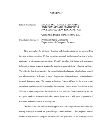
Submodular Dictionary Selection for Sparse Representationcombinatorial challenges, the existing dictionary learning work relies on continuous relaxations, such as replacing the combinatorial sparsity constraint with the 1 -norm of the dictionary representation of the signal.However, these approaches result in non-convex objectives, and the performance of such relaxations is typically not well-characterized for dictionary learning.3. Submodularity in sparserepresentationApproximate submodularity in DiSP: To definethis concept, we first note that F ( ) 0 and whenever D D0 then F (D) F (D0 ), i.e., F increasesmonotonically with D. In the sequel, we will showthat F is approximately submodular: A set functionF is called approximately submodular with constant ε,if for D D0 V and v V \ D0 it holds thatF (D {v}) F (D) F (D0 {v}) F (D0 ) ε. (5)In the context of DiSP, the above definition impliesthat adding a new column v to a larger dictionary D0helps at most ε more than adding v to a subset D D0 .When ε 0, the set function is called submodular.A fundamental result by Nemhauser et al. (1978)proves that for monotonic submodular functions Gwith G( ) 0, a simple greedy algorithm that startswith the empty set D0 , and at every iteration iadds a new element via(6)v V\Dwhere Di {v1 , . . . , vi }, obtains a near-optimal solution. That is, for the solution Dn returned by thegreedy algorithm, we have the following guarantee:G(Dn ) (1 1/e) max G(D). D n(7)The solution Dn hence obtains at least a constant fraction of (1 1/e) 63% of the optimal value.Using similar arguments, Krause et al. (2008) showthat the same greedy algorithm, when applied to approximately submodular functions, instead inheritsthe following–slightly weaker–guaranteeF (Dn ) (1 1/e) max F (D) nε. D n(8)sin(ψ θ)ysys1/2ws,vψcos( ψ θ)ψθys {A}In this section, we first describe a key structure in theDiSP objective function: approximate submodularity.We then relate this structure to a geometric propertyof the candidate vector set, called incoherence. We usethese two concepts to develop efficient algorithms withprovable guarantees in the next section.vi argmax G(Di 1 {v}),vvys {v}sin(θ)θcos(θ)A1/2Aws,AFigure 1. Example geometry in DiSP. (Left) Minimum error decomposition. (Right) Modular decomposition.Geometry in DiSP (incoherence): The approximate submodularity of F explicitly depends on themaximum incoherency µ of ΦV [φ1 , . . . , φN ]:µ max hφi , φj i (i,j),i6 jmax cos ψi,j , (i,j),i6 jwhere ψi,j is the angle between the vectors φi and φj .The following lemma establishes a key relationship between ε and µ for DiSP.Theorem 1 If ΦV has incoherence µ, then the variance reduction objective F in DiSP is ε-approximatelysubmodular with ε 4kµ.Proof Let ws,v hφv , ys i2 . When ΦV is an orthonormal basis, the reconstruction accuracy in (1) can bewritten as followsQXX2Ls (A) ys φiq hys , φiq i ys 22 ws,v .2q 1v AHencethe function Rs (A) Ls ( ) Ls (A) Pv A ws,v is additive (modular). It can be seen thatthen Fs (D) maxA D, A k Rs (A) is submodular.Now suppose ΦV is incoherent with constant µ. LetA V and v V \ A. Then we claim that Rs (A {v}) Rs (A) ws,v µ. Consider the special case where ys is in the span of two subspaces Aand v, and w.l.o.g., ys 2 1; refer to Fig. 1 for anillustration. The reconstruction accuracy as definedin (1) has a well-known closed form solution: Ls (A) minw ys ΦA w 22 ys ΦA Φ†A ys 22 , where † denotesthe pseudoinverse; the matrix product P ΦA Φ†A issimply the projection of the signal ys onto the subspace of A. We therefore have Rs (A) 1 sin2 (θ),Rs (A {v}) 1, and Rs ({v}) 1 sin2 (ψ θ), whereθ and ψ are defined in Fig. 1. We thus can boundεs Rs (A {v}) Rs (A) wv,s byεs max sin2 (ψ θ) sin2 (θ) 1θ cos ψ max cos(ψ 2θ) µ.θIn Section 4, we explain how this greedy algorithm canbe adapted to DiSP. But first, we elaborate on how εdepends on the candidate vector set ΦV .If ys is not in the span of A {v}, we apply abovereasoning to the projection of ys onto their span.

Submodular Dictionary Selection for Sparse Representationbs (A) PDefine RThen, by induction,v A ws,v .bs (A) Rs (A) kµ. Note that thewe have Rbs (A) is submodufunction Fbs (D) maxA D, A k Rlar. Let As argmaxA D, A k Rs (A) and Abs bs (A). Therefore, it holds thatargmaxA D, A k Rb s ) kµ R(b Abs ) kµ Fbs (D) kµ.Fs (D) Rs (As ) R(ASimilarly, Fbs (D) Fs (D) kµ. Thus, Fbs (D) Fs (D) kµ, and hence Fb(D) F (D) kµ holdsfor all candidate dictionaries D. Therefore, wheneverD D0 and v / D0 , we can obtain the followingF (D {v}) F (D) F (D0 {v}) F (D0 ) Fb(D {v}) Fb(D) Fb(D0 {v}) Fb(D0 ) 4kµ 4kµ, which proves the claim.When the incoherency µ is small, the approximationguarantee in (8) is quite useful. There has been a significant body of work establishing the existence andconstruction of collections V of columns with low coherence µ. For example, it is possible to achieve incoherence µ d 1/2 with the union of d/2 orthonormalbases (c.f. Theorem 2 of Gribonval & Nielsen (2002)).Unfortunately, when n Ω(d) and ε 4kµ, the guarantee (8) is vacuous since the maximum value of F forDiSP is 1. In Section 4, we will show that if, instead ofgreedily optimizing F , we optimize a modular approximation Fbs of Fs (as defined below), we can improvethe approximation error from O(nkµ) to O(kµ).A modular approximation to DiSP: The keyidea behind the proof of Theorem 1 is that for incoherent dictionaries the variance reduction Rs (A) Ls ( ) Ls (A) is approximately additive (modular).We exploit this observation by optimizing a new objective Fb that approximates F by disregarding the nonorthogonality of ΦV in sparse representation. We dothis by replacing the weight calculation ws,A Φ†A ysin F with ws,A ΦTA ys :X1 XbFbs (D) maxws,v , and Fb(D) Fs (D),m sA D, A kv A(9)where ws,v hφv , ys i2 for each ys Rd and φv ΦV .We call Fb a modular approximation of F as it relies onthe approximate modularity of the variance reductionRs . Note that in contrast to (3), Fbs (D) in (9) can beexactly evaluated by a greedy algorithm that simplypicks the k largest weights ws,v . Moreover, the weightsmust be calculated only once during algorithm execution, thereby significantly increasing its efficiency.The following immediate Corollary to Theorem 1 summarizes the essential properties of Fb:Corollary 1 Suppose ΦV is incoherent with constantµ. Then, for any D V, we have Fb(D) F (D) kµ.Furthermore, Fb is monotonic and submodular.Corollary 1 shows that Fb is a close approximation ofthe DiSP set function F . We exploit this modular approximation to motivate a new algorithm for DiSP andprovide better performance bounds in Section 4.4. Sparsifying dictionary selectionIn this section, we describe two sparsifying dictionaryselection (SDS) algorithms with theoretical performance guarantees: SDSOM P and SDSM A . Both algorithms make locally greedy choices to handle the combinatorial challenges C1 and C2, defined in Section 2.The algorithms differ only in the way they addressC1, which we further describe below. Both algorithmstackle C2 by the same greedy scheme in (6). That is,both algorithms start with the empty set and greedilyadd dictionary columns to solve DiSP. Interestingly,while SDSM A has better theoretical guarantees andis much faster than SDSOM P , Section 6 empiricallyshows that SDSOM P often performs better.SDSOM P : SDSOM P employs the orthogonal matching pursuit (OMP) (Gilbert & Tropp, 2005) to approximately solve the sparse representation problem in (2)and has the following theoretical guarantee:Theorem 2 SDSOM P uses the scheme in (6) to builda dictionary DOMP one column at a time such thatF (DOMP ) (1 1/e) max F (D) k(6n 2 1/e)µ. D nBefore we prove Theorem 2, we state the followingresult whose proof directly follows from Theorem 1.Proposition 1 At each iteration, SDSOM P approximates F with a value FOM P such that FOM P (D) F (D) kµ over all dictionaries D.Proof [Theorem 2] From Theorem 1 and Proposition 1we can see that FOM P is 6knµ-approximately submodular. Thus, according to Krause et al. (2008):FOM P (DOMP ) (1 1/e) max FOM P (D) 6knµ. D n(10)Using Proposition 1, we substitute F (DOMP ) kµ FOM P (DOMP ) and max D n FOM P (D) max D nF (D) kµ into (10) to prove the claim.SDSM A : SDSM A greedily (according to (6)) optimizes the modular approximation (MA) Fb of the DiSPobjective F and has the following guarantee:Theorem 3 SDSM A builds a dictionary DMA s.t.F (DM A ) (1 1/e) max F (D) (2 1/e)kµ. (11) D nCorollary 1 and Theorem 2 directly imply Theorem 3.

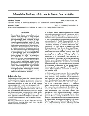
Submodular Dictionary Selection for Sparse RepresentationIn most realistic settings with high-dimensional signalsand incoherent dictionaries, the term (2 1/e)kµ in theapproximation guarantee (11) of SDSM A is negligible.5. Sparsifying dictionary selectionfor block sparse representationStructured sparsity: While many man-made andnatural signals can be described as sparse in simpleterms, their sparse coefficients often have an underlying, problem dependent order. For instance, modern image compression algorithms, such as JPEG, notonly exploit the fact that most of the DCT coefficientsof a natural image are small. Rather, they also exploit the fact that the large coefficients have a particular structure characteristic of images containing edges.Coding this structure using an appropriate model enables transform coding algorithms to compress imagesclose to the maximum amount possible and significantly better than a naive coder that just assigns bitsto each large coefficient independently (Mallat, 1999).We can enforce structured sparsity for sparse coefficients over the learned dictionaries in DiSP, corresponding to a restricted union-of-subspaces (RUS)sparse model by imposing the constraint that the feasible sparsity patterns are a strict subset of all kdimensional subspaces (Baraniuk et al., 2008). To facilitate such RUS sparse models in DiSP, we must notonly determine the constituent dictionary columns,but also their arrangement within the dictionary.While analyzing the RUS model in general is challenging, we here describe below a special RUS model ofbroad interest to explain the general ideas.Block-sparsity: Block-sparsity is abundant inmany applications. In sensor networks, multiplesensors simultaneously observe a sparse signal overa noisy channel. While recovering the sparse signaljointly from the sensors, we can use the fact that thesupport of the significant coefficients of the signal arecommon across all the sensors. In DNA microarrayapplications, specific combinations of genes arealso known a priori to cluster over tree structures,called dendrograms. In computational neuroscienceproblems, decoding of natural images in the primaryvisual cortex (V1) and statistical behavior of neuronsin the retina exhibit clustered sparse responses.To address block-sparsity in DiSP, we replace (3) byXXFi (D) Ls ( ) minLs (A), (12)s BiA D, A ks Biwhere Bi is the i-th block of signals (e.g., simultaneous recordings by multiple sensors) that must sharethe same Psparsity pattern. Accordingly, we redefineF (D) i Fi (D) as the sum across blocks, ratherthan individual signals, as Section 6 further elaborates.This change preserves (approximate) submodularity.6. ExperimentsFinding a dictionary in a haystack: To understand how the theoretical performance reflects on theactual performance of the proposed algorithms, wefirst perform experiments on synthetic data.We generate a collection VU with 400 columns by forming a union of six orthonormal bases with d 64,including the discrete cosine transform (DCT), different wavelet bases (Haar, Daub4, Coiflets), noiselets, and the Gabor frame. This collection VU is notincoherent—in fact, the various bases contain perfectlycoherent columns. As alternatives, we first create aseparate collection VS from VU , where we greedily removed columns based on their incoherence, until theremaining collection had incoherence of µS 0.5. Theresulting collection contains 245 columns. We also create a collection VR with 150 random columns of VU ,which results in µR 0.23.For VU,S,R , we repeatedly (50 trials) pick at randoma dictionary D V of size n 64 and generate acollection of m 100 random 5-sparse signals withrespect to the dictionary D . Our goal is to recoverthe true dictionary D using our SDS algorithms. Foreach random trial, we run SDSOM P and SDSM A toselect a dictionary D of size 64. We then look at theoverlap D D to measure the performance of selecting the “hidden” basis D . We also report the fractionof remaining variance after sparse reconstruction.Figures 2(a), 2(b), and 2(c) compare SDSOM P andSDSM A in terms of their variance reduction as a function of the selected number of columns. Interestingly,in all 50 trials, SDSOM P perfectly reconstructs thehidden basis D when selecting 64 columns for VS,R .SDSM A performs slightly worse than SDSOM P .Figures 2(e), 2(f), and 2(g) compare the performancein terms of the fraction of incorrectly selected basisfunctions. Note that, as can be expected, in case ofthe perfectly coherent VU , even SDSOM P does notachieve perfect recovery. However, even with high coherence, µ 0.5 for VS , SDSOM P exactly identifiesD . SDSM A performs a slightly worse but nevertheless correctly identifies a high fraction of D .In addition to exact sparse signals, we also generate compressible signals, where the coefficients havepower-law with decay rate of 2. These signals canbe well-approximated as sparse; however, the residualerror in sparse representation creates discrepancies inmeasurements which can be modeled as noise in DiSP.Figures 2(d) and 2(h) repeat the above experiments forVS ; both SDSOM P and SDSM A perform quite well.

(a) VU 80.60.40.200SDSMA0.40.2SDSMA0.80.60.40.2(f) VS –sparse0.08SDSOMP(g) VR –sparseResidual varianceRunning time (s)0110210Dimension310(i) Dimension vs. runtimeMA0.060.040.0200.10.20.3Incoherence µ0.4(j) Incoherence vs. res. var.SDSMA0.020.0150.010.0050 210SDSMA0.60.40.20050100# columns selected(d) VS SSDSMASDSOMP0.80050100# columns selected0.025SDS11SDSOMP0050100# columns selected50100# columns selected(c) VR –sparse10.6(e) VU –sparse10 010(b) VS –sparseSDSOMP0050100# columns selected51050100# columns selectedResidual variance0.850100# columns selected0.6SDSOMPFraction of remaining variance000.81Fraction of incorrect atoms0.2SDSMAFraction of incorrect atoms0.4SDSOMPFraction of remaining variance0.61Fraction of incorrect atomsSDSMA0.81Fraction of incorrect atomsSDSOMPFraction of remaining variance1Fraction of incorrect atomsFraction of remaining varianceSubmodular Dictionary Selection for Sparse Representation310Number of signals(k) # Signals vs. res. var.0.80.650100# columns selected(h) VS –compressibleSDSOMPSDSMASDSMAB0.40.20050100# columns selected(l) Block-sparseFigure 2. Results of 50 trials: (a-c) Variance reduction achieved by SDSOM P and SDSM A on the collections VU,S,R for5-sparse signals in 64 dimensions. (e-g) Percentage of incorrectly selected columns on the same collections. (d) Variancereduction for compressible signals in 64 dimensions for VS . (h) Corresponding column selection performance. (i) SDSM Ais orders of magnitude faster than SDSOM P over a broad range of dimensions. (j) As incoherence decreases, the algorithmeffectiveness in variance reduction improve. (k) The variance reduction performance of SDSM A improves with the numberof training samples. (l) Exploiting block-sparse structure in signals leads to improved dictionary selection performance.Figure 2(i) compares SDSOM P and SDSM A in running time. As we increase the dimensionality of theproblem, SDSM A is several orders of magnitude fasterthan SDSOM P in our MATLAB implementation. Figure 2(j) illustrates the performance of the algorithmsas a function of the incoherence. As predicted by Theorems 2 and 3, lower incoherence µ leads to improvedperformance of the algorithms. Lastly, Figure 2(k)compares the residual variance as a function of thetraining set size (number of signals). Surprisingly,as the number of signals increase, the performance ofSDSM A improves, and even exceeds that of SDSOM P .We also test the extension of SDSM A to block-sparsesignals as discussed in Section 5. We generate 200random signals each with fixed sparsity pattern, comprising 10 blocks, consisting of 20 signals each. Wethen compare the standard SDSM A algorithm withthe block-sparse variant SDSM AB described in Section 5 in terms of their basis identification performance (see Figure 2(l)). SDSM AB drastically outperforms SDSM A , and even outperforms the SDSOM Palgorithm which is computationally far more expensive. Hence, exploiting prior knowledge of the problemstructure can significantly aid dictionary selection.A battle of bases on image patches: In this experiment, we try to find the optimal dictionary amongan existing set of bases to represent natural images.Since the conventional dictionary learning approachescannot be applied to this problem, we only present theresults of SDSOM P and SDSM A .We sample image patches from natural images, andapply our SDSOM P and SDSM A algorithms to selectdictionaries from the collection VU , as defined above.Figures 3(a) (for SDSOM P ) and 3(b) (for SDSM A )show the fractions of selected columns allocated to thedifferent bases constituting VU for 4000 image patchesof size 8 8. We restrict the maximum number ofdictionary coefficients k for sparse representation to10% (6). We then observe the following surprisingresults. While wavelets are considered to be animprovement over the DCT basis for compressingnatural images (JPEG2000 vs. JPG), SDSOM P prefer

Submodular Dictionary Selection for Sparse Representation0.60.40.20050100Number of columns150(a) Bases used (SDSOM P ber of columns150(b) Bases used (SDSM A )Gabor0.80.6Daub4HaarDCT0.40.20Fraction per basis0.8111Fraction of residual varianceDCTHaarDaub4Coif1NoiseGaborFraction per basisFraction per basis1SDSOMP2040Number of columns60(c) Test set var. 50010001500Number of columns2000(d) Bases used (SDSM A )Figure 3. Experiments on natural image patches. (a,b,c) Fractions of bases selected for SDSOM P and SDSM A with d 64(a,b), and the corresponding variance reduction on test patches. (d) Fractions of bases selected for SDSM A with d 1024.DCT over wavelets for sparse representation; the crossvalidation results show that the learned combinationof DCT (global) and Gabor functions (local) are betterthan the wavelets (multiscale) in variance reduction(compression). In particular, Fig. 3(c) demonstratesthe performance of the learned dictionary against thevarious bases that comprise VU on a held-out testset of 500 additional image patches. The variancereduction of the dictionary learned by SDSOM P is8% lower than the variance reduction achieved by thebest basis, which, in this case, is DCT.Moreover, SDSM A , which trades off representationaccuracy with efficient computation, overwhelminglyprefers Gabor functions that are used to model neuronal coding of natural images. The overall dictionaryconstituency varies for SDSOM P and SDSM A ; however, the variance reduction performances are comparable. Finally, Figure 3(d) presents the fraction of selected bases for 32 32 sized patches with k 102,which matches well with the 8 8 DiSP problem above.Dictionary selection from dimensionality reduced data: In this experiment, we focus on a specific image processing problem, inpainting, to motivate a dictionary selection problem from dimensionality reduced data. Suppose that instead of observing Y as assumed in Section 2, we observe Y 0 P1 y1 , . . . , Pm ym Rb , where Pi Rb d i are knownlinear projection matrices. In the inpainting setting,Pi ’s are binary matrices which pass or delete pixels.From a theoretical perspective, dictionary selectionfrom dimensionality reduced data is ill-posed. For thepurposes of this demonstration, we will assume thatPi ’s are information preserving.As opposed to observing a series of signal vectors,we start with a single image in Fig. 4, albeit missing50% of its pixels. We break the noisy image intonon-overlapping 8 8 patches, and train a dictionaryfor sparse reconstruction of those patches to minimizethe average approximation error on the observedpixels. As candidate bases, we use DCT, wavelets(Haar and Daub4), Coiflets (1 and 3), and Gabor.We test our SDSOM P and SDSM A algorithms,approaches based on total-variation (TV), linearinterpolation, nonloc

characterizations of the dictionary design approaches. In this paper, we investigate a hybrid approach be-tween dictionary design and learning. We propose a learning framework based on dictionary selection: We build a sparsifying dictionary for a set of observations by selecting the dictionary columns from multiple can-