Transcription
DS288-Numerical MethodsUE201-Introduction to Scientific ComputingRatikanta BeheraDepartment of computational and Data Sciences,Indian Institute of Science BangaloreAugust-December 2022Ratikanta BeheraDS288/UE201Lecture-1 (August 04, 2022)1 / 17
BooksNumerical Methods/ Introduction to Scientific ComputingNumerical Analysis (Richard L. Burden & J. Douglas Faires)Numerical Methods with MATLAB (G. J. Borse)Numerical Recipes in C/FORTRAN (Press, Teukolsky, Vetterling,and Flannery)Elementary Numerical Analysis (Kendall Atkinson & Weimin Han).Ratikanta BeheraDS288/UE201Lecture-1 (August 04, 2022)2 / 17
Scientific Computing Scientific Computing is the collection of tools, techniques, andtheories required to solve mathematical models of problems inScience and Engineering on a computer.Ratikanta BeheraDS288/UE201Lecture-1 (August 04, 2022)3 / 17
Scientific Computing Scientific Computing is the collection of tools, techniques, andtheories required to solve mathematical models of problems inScience and Engineering on a computer. It is a third pillar of science, standing right next to theoreticalanalysis and experiments.Ratikanta BeheraDS288/UE201Lecture-1 (August 04, 2022)3 / 17
Scientific Computing Scientific Computing is the collection of tools, techniques, andtheories required to solve mathematical models of problems inScience and Engineering on a computer. It is a third pillar of science, standing right next to theoreticalanalysis and experiments. Why Scientific Computing ?Ratikanta BeheraDS288/UE201Lecture-1 (August 04, 2022)3 / 17
Scientific Computing Scientific Computing is the collection of tools, techniques, andtheories required to solve mathematical models of problems inScience and Engineering on a computer. It is a third pillar of science, standing right next to theoreticalanalysis and experiments. Why Scientific Computing ?Trying to predict climate change.When experiments dangerous, too large, too expensive, critical.Ratikanta BeheraDS288/UE201Lecture-1 (August 04, 2022)3 / 17
Scientific Computing Scientific Computing is the collection of tools, techniques, andtheories required to solve mathematical models of problems inScience and Engineering on a computer. It is a third pillar of science, standing right next to theoreticalanalysis and experiments. Why Scientific Computing ?Trying to predict climate change.When experiments dangerous, too large, too expensive, critical. Scientific computing draws on mathematics and computerscience to develop the best way to use computer to solveproblems in science and engineering.Ratikanta BeheraDS288/UE201Lecture-1 (August 04, 2022)3 / 17
Scientific Computing Scientific Computing is the collection of tools, techniques, andtheories required to solve mathematical models of problems inScience and Engineering on a computer.Ratikanta BeheraDS288/UE201Lecture-1 (August 04, 2022)4 / 17
Scientific Computing Scientific Computing is the collection of tools, techniques, andtheories required to solve mathematical models of problems inScience and Engineering on a computer. This set of mathematical theories and techniques is calledNumerical Mathematics or Numerical Methods.Ratikanta BeheraDS288/UE201Lecture-1 (August 04, 2022)4 / 17
Scientific Computing Scientific Computing is the collection of tools, techniques, andtheories required to solve mathematical models of problems inScience and Engineering on a computer. This set of mathematical theories and techniques is calledNumerical Mathematics or Numerical Methods. Numerical methods are procedures that allow for efficientsolution of a mathematically formulated problem in a finitenumber of steps to within an arbitrary precision.Ratikanta BeheraDS288/UE201Lecture-1 (August 04, 2022)4 / 17
Scientific Computing Scientific Computing is the collection of tools, techniques, andtheories required to solve mathematical models of problems inScience and Engineering on a computer. This set of mathematical theories and techniques is calledNumerical Mathematics or Numerical Methods. Numerical methods are procedures that allow for efficientsolution of a mathematically formulated problem in a finitenumber of steps to within an arbitrary precision. Numerical methods commonly consist of a set of guidelines toperform predetermined mathematical operations (algebraic andlogical) leading to an approximate solution of a specific problem.such set of guidelines is know as an algorithm.Ratikanta BeheraDS288/UE201Lecture-1 (August 04, 2022)4 / 17
Scientific Computing ProcessRatikanta BeheraDS288/UE201Lecture-1 (August 04, 2022)5 / 17
Scientific Computing Process Represent Mathematical Model:Ratikanta BeheraDS288/UE201Lecture-1 (August 04, 2022)6 / 17
Scientific Computing Process Represent Mathematical Model: Express the Working Modelin mathematical terms; write down mathematical equations oran algorithm whose solution describes the Working Model . In general, the success of a mathematical model depends on howeasy it is to use and how accurately it predicts.Ratikanta BeheraDS288/UE201Lecture-1 (August 04, 2022)6 / 17
Scientific Computing Process Translate Computational Model:Ratikanta BeheraDS288/UE201Lecture-1 (August 04, 2022)7 / 17
Scientific Computing Process Translate Computational Model: Change MathematicalModel into a form suitable for computational solution. Computational models include languages, such as Python, C or Java, or software, like Matlab or Mathematica.Ratikanta BeheraDS288/UE201Lecture-1 (August 04, 2022)7 / 17
Scientific Computing Process Simulate Results/Conclusions:Ratikanta BeheraDS288/UE201Lecture-1 (August 04, 2022)8 / 17
Scientific Computing Process Simulate Results/Conclusions: Run Computational Model toobtain Results; draw Conclusions. Verify your computer program; use check cases; explore rangesof validity. Sometime, Graphs, charts, and other visualizationtools are useful in summarizing results and drawing conclusions.Ratikanta BeheraDS288/UE201Lecture-1 (August 04, 2022)8 / 17
Numerical Calculation vs Symbolic CalculationNumerical Calculation:Ratikanta BeheraDS288/UE201Lecture-1 (August 04, 2022)9 / 17
Numerical Calculation vs Symbolic CalculationNumerical Calculation: (involve numbers directly) Manipulatenumbers to produce a numerical result Example:(17.36)2 1 16.36(1)17.36 1Symbolic Calculation:Ratikanta BeheraDS288/UE201Lecture-1 (August 04, 2022)9 / 17
Numerical Calculation vs Symbolic CalculationNumerical Calculation: (involve numbers directly) Manipulatenumbers to produce a numerical result Example:(17.36)2 1 16.36(1)17.36 1Symbolic Calculation: (symbols represent numbers) Manipulate symbols according to mathematical rules to producea symbolic result Example:x2 1 x 1(2)x 1Ratikanta BeheraDS288/UE201Lecture-1 (August 04, 2022)9 / 17
Analytic Solution Vs Numerical SolutionAnalytic Solution:Ratikanta BeheraDS288/UE201Lecture-1 (August 04, 2022)10 / 17
Analytic Solution Vs Numerical SolutionAnalytic Solution: The exact numerical/symbolic representationof the solution. It may use special characters such as1 1, , 7π, e, or tan(83)4 5(3)Numerical Solution:Ratikanta BeheraDS288/UE201Lecture-1 (August 04, 2022)10 / 17
Analytic Solution Vs Numerical SolutionAnalytic Solution: The exact numerical/symbolic representationof the solution. It may use special characters such as1 1, , 7π, e, or tan(83)4 5(3)Numerical Solution: The computational representation of thesolution. It is entirely numericalExample:.25, 0.33333 · · · , 3.14159 · · · , 0.88472 · · ·Ratikanta BeheraDS288/UE201Lecture-1 (August 04, 2022)10 / 17
Floating point representationA non-zero real number x to be stored in the computer of the formx (0.a1 a2 a3 · · · ak ) 10n(4)where 1 a1 9, and 0 ai 9, i 2, 3, · · · , k 10 base number. n an integer called exponent (positive or negative or zero) 0.a1 a2 a3 · · · ak mantissaHere the Eq. (4) is called normalized k decimal floating point form.ExampleNormalized decimal representation the following numbers12345.67 0.1234567 1050.00123 0.123 10 2Ratikanta BeheraDS288/UE201Lecture-1 (August 04, 2022)(5)(6)11 / 17
Significant FiguresSignificant figures are the number of digits in a value that are knownwith some degree of confidence, often a measurement, thatcontribute to the degree of accuracy of the value. All non zero digits are significant. 549 has three significant figures 1.892 has four significant figuresRatikanta BeheraDS288/UE201Lecture-1 (August 04, 2022)12 / 17
Significant FiguresSignificant figures are the number of digits in a value that are knownwith some degree of confidence, often a measurement, thatcontribute to the degree of accuracy of the value. All non zero digits are significant. 549 has three significant figures 1.892 has four significant figures Zeros between non zero digits are significant. 4023 has four significant figures 50014 has five significant figuresRatikanta BeheraDS288/UE201Lecture-1 (August 04, 2022)12 / 17
Significant FiguresSignificant figures are the number of digits in a value that are knownwith some degree of confidence, often a measurement, thatcontribute to the degree of accuracy of the value. All non zero digits are significant. 549 has three significant figures 1.892 has four significant figures Zeros between non zero digits are significant. 4023 has four significant figures 50014 has five significant figures Zeros to the left of the first non zero digit are not significant. 0.000034 has only two significant figures. (as it is 3.4x10 5 ) 0.001111 has four significant figures.Ratikanta BeheraDS288/UE201Lecture-1 (August 04, 2022)12 / 17
Significant Figures Trailing zeros (the right most zeros) are significant when there isa decimal point in the number. 400. Ratikanta BeheraDS288/UE201Lecture-1 (August 04, 2022)13 / 17
Significant Figures Trailing zeros (the right most zeros) are significant when there isa decimal point in the number. 400. has three significant figures 2.00 Ratikanta BeheraDS288/UE201Lecture-1 (August 04, 2022)13 / 17
Significant Figures Trailing zeros (the right most zeros) are significant when there isa decimal point in the number. 400. has three significant figures 2.00 has three significant figures 0.050 Ratikanta BeheraDS288/UE201Lecture-1 (August 04, 2022)13 / 17
Significant Figures Trailing zeros (the right most zeros) are significant when there isa decimal point in the number. 400. has three significant figures 2.00 has three significant figures 0.050 has two significant figures Trailing zeros are not significant in numbers without decimalpoints. 470000 Ratikanta BeheraDS288/UE201Lecture-1 (August 04, 2022)13 / 17
Significant Figures Trailing zeros (the right most zeros) are significant when there isa decimal point in the number. 400. has three significant figures 2.00 has three significant figures 0.050 has two significant figures Trailing zeros are not significant in numbers without decimalpoints. 470000 has two significant figures 400 (or 4 102 ) indicates only one significant figure.Remark: To indicate that the trailing zeros are significant a decimal pointmust be added.Ratikanta BeheraDS288/UE201Lecture-1 (August 04, 2022)13 / 17
Approximation of numbersMost real numbers x cannot be represented exactly by thenormalized decimal floating-point form.We approximate by a nearby number to represent in a computer. Translating a real number x into k-digit floating point numberSuppose we want to round off the number (Rounding or Chopping)x (0.a1 a2 a3 · · · ak ak 1 · · · ) 10n with a1 ̸ 0 let fl(x) denote its normalized decimal floating-point form. Thenfl(x) (0.a1 a2 a3 · · · ak ) 10n whereak akif ak ak 1 ifRatikanta BeheraDS288/UE201ak 1 5 and5 ak 1Lecture-1 (August 04, 2022)14 / 17
ERRORThe following types of error will come for any numerical computation.Inherent error:Ratikanta BeheraDS288/UE201Lecture-1 (August 04, 2022)15 / 17
ERRORThe following types of error will come for any numerical computation.Inherent error: Errors which are already present in the statementof the problem before its solution.Rounding error:Ratikanta BeheraDS288/UE201Lecture-1 (August 04, 2022)15 / 17
ERRORThe following types of error will come for any numerical computation.Inherent error: Errors which are already present in the statementof the problem before its solution.Rounding error: Arise from the process of rounding off thenumbers during the computations.Truncation error:Ratikanta BeheraDS288/UE201Lecture-1 (August 04, 2022)15 / 17
ERRORThe following types of error will come for any numerical computation.Inherent error: Errors which are already present in the statementof the problem before its solution.Rounding error: Arise from the process of rounding off thenumbers during the computations.Truncation error: This errors are caused by using approximateresults or replacing an infinite process by a finite one. (type ofalgorithm error)Absolute, Relative and Percentage errorsRatikanta BeheraDS288/UE201Lecture-1 (August 04, 2022)15 / 17
Absolute, Relative and Percentage errors Consider X true value of the quantity and X ′ approximate valueAbsolute error, Ea X X ′ Relative error, Er X X ′ X XPercentage error, Ep 100Er 100 X X ′ RemarkThe relative and percentage error are independent of unit.Absolute error is expressed in terms of these unit.Ratikanta BeheraDS288/UE201Lecture-1 (August 04, 2022)16 / 17
Ratikanta BeheraDS288/UE201Lecture-1 (August 04, 2022)17 / 17
Numerical Methods/ Introduction to Scientific Computing Numerical Analysis(Richard L. Burden & J. Douglas Faires) . Science and Engineering on a computer. It is athird pillar of science, standing right next totheoretical . Computational models include languages, such as Python, C or Java, or software, like Matlab or Mathematica. .