Transcription
Simultaneous Planning for New Product Development and BatchManufacturing FacilitiesChristos T. Maravelias and Ignacio E. Grossmann Department of Chemical EngineeringCarnegie Mellon UniversityPittsburgh, PA 15213ABSTRACTOne of the greatest challenges in highly regulated industries, such as pharmaceuticals and agrochemicals, is theprocess of selecting, developing and efficiently manufacturing new products that emerge from the discoveryphase. This process involves the performance of regulatory tests, such as environmental and safety tests, for thenew products, and the plant design for manufacturing the products that pass all tests. In order to systematicallyaddress this problem, we consider the simultaneous optimization of resource-constrained scheduling of testingtasks in new product development, and design/planning of batch manufacturing facilities. A multiperiodmixed-integer linear programming (MILP) model that maximizes the expected net present value of multipleprojects is proposed. The model takes into account multiple trade-offs and predicts which products should betested, the detailed test schedules that satisfy resource constraints, design decisions for the process network,and production profiles for the different scenarios defined by the various testing outcomes. In order to solvelarger instances of this problem with reasonable computational effort, a heuristic algorithm based onLagrangean decomposition is proposed. The algorithm exploits the special structure of the problem andcomputational experience shows that it provides optimal or near optimal solutions, while being significantlyfaster than the full space method. The application of the model is illustrated with three example problems.IntroductionA large number of candidate new products in the agricultural and pharmaceutical industry must undergo a setof tests related to safety, efficacy, and environmental impact, in order to obtain certification. Depending on thenature of the products, testing may last up to 5 years, and their scheduling should be made with the goal ofminimizing the time to market and the cost of the testing. In order to be competitive, a company must have anumber of promising products at different stages of the testing process, and at the same time must be preparedto produce a new product as soon as testing is successfully completed. Since the building of a new plant, thespecification and procuring of equipment, and the validation process last more than two years, an investmentdecision for the manufacturing of the new product(s) must be made well before testing is completed.Furthermore, investment decisions become even more important as the pressures for reducing the costs ofpharmaceutical products increase. Clearly, the timing of these decisions depends on the completion time oftesting of new product(s), and the size of investment depends on the number of new products and theirproduction levels. Thus, given these complex trade-offs, decisions on the testing of new products, and on thedesign and planning of manufacturing facilities should be optimized simultaneously.Although optimization methods for addressing problems separately in new product development1,2,3,4,5,6,7 andsupply chain management8,9,10,11,12 have been reported in the literature, the integrated problem addressed in thispaper does not appear to have been reported before. Currently there are no methods and tools to explicitlyaddress this problem, and in practice, decisions are made on an ad-hoc basis. A new optimization model foraddressing this design integration problem is presented in this paper. The proposed model is a large-scale Author to whom correspondence should be addressed.E-mail: grossmann@andrew.cmu.edu. Phone: 412-268-2230. Fax: 412-268-7139
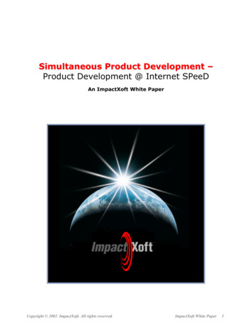
2MILP that predicts, from a portfolio of potential new products, which products should be tested, the detailedtest schedules, design decisions for the process network, and production profiles of existing and new products.Since the integration leads to a very large and hard MILP problem to solve, a solution method based on aheuristic Lagrangean decomposition is also proposed.Literature ReviewSchmidt and Grossmann3 proposed several optimization models for the optimal scheduling of testing tasks inthe new product development process, and Jain and Grossmann4 extended these models to take into accountresource constraints. Honkomp et al.5 addressed the problem of selecting process development projects from apool of projects, and scheduling the use of limited resources to maximize the expected return from researchand development operations. This problem is similar to the scheduling of testing tasks, as each processdevelopment project requires a specific sequence of tasks, each of which has a probability of failure.Subramanian et al.6 proposed a simulation-based framework for the management of the R&D pipeline, andBlau et al.7 developed a simulation model for risk management in the new product development process. Thefocus of these references, however, is the new product development process, and not the design and planningof manufacturing facilities. In most of these references it is assumed, for instance, that there are no capacitylimitations, or that the production level of a new product is not affected by the production levels of otherproducts. Furthermore, investment costs are not explicitly included in the calculation of Net Present Value(NPV) of projects. Papageorgiou et al.10 proposed an optimization-based approach for selecting from a set ofcandidate products the ones to be commercialized. Their approach includes a capacity planning strategy, butdoes not account for the testing tasks that need to be performed for certification.There is a large number of papers on batch design (Reklaitis13) that deal with detailed sizing and scheduling.Norton and Grossmann13 proposed a simplified high level, multiperiod planning investment model forprocessing networks with dedicated and flexible plants. This model is a multiperiod mixed-integer linearprogramming model, which for given forecasts of product demands and pricing, maximizes the net presentvalue of processing network’s operations and expansion decisions over a long time horizon. In that model, it isassumed that products are known and that all products can be produced immediately. In contrast, in theproblem addressed in this paper, from a given portfolio of potential products, only a few will be selected to betested and produced if they pass all tests successfully.In this work we develop a new integrated scheduling and planning model that uses as a basis the schedulingmodel of Jain and Grossmann4, and the design/planning model of Norton and Grossmann13. Jain andGrossmann4 assumed that all potential products are to be tested. However, in this work one has to decide whichproducts should be tested, since there might not be enough testing facilities, or not all products may beprofitable. Therefore, the proposed model must select which products to test. In order to account for thisdecision we use disjunctive programming. If a product is selected to be tested, all the constraints that describeresource-constrained scheduling are active; if it is not selected, all variables referring to testing of this productare set to zero. In most planning models (e.g. Norton and Grossmann13) it is assumed that the level of sales islimited by plant capacity and demand (which is either known or uncertain within a fixed range). In newproduct development, however, the production of a potential product depends also on whether this product hasbeen selected and has passed all tests. This is a discrete-state type of uncertainty, which has received littleattention in the literature (Straub and Grossmann14). It is, therefore, necessary to extend planning models toaccount for discrete uncertainties, which will be done in this paper with the use of scenarios.RepresentationFor the representation of testing schedules, we use Gantt charts from the perspective of resources to display theuse of each resource over time, and activity-on-node directed graphs to display the optimal sequence of tasks.To illustrate, consider the example of a product X that requires four tests and resources from two categories.Tests 1 and 2 require resource A and tests 3 and 4 require resource B. There are also technological precedence
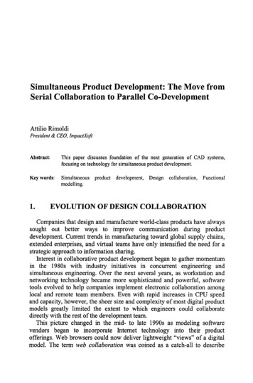
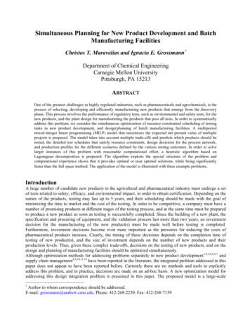
3constraints: test 1 must finish before tests 3 and 4 begin. Using the proposed representations, a solution to thisproblem is presented in Figure 1. TX is the completion time of testing of product X.12TX2Res A4Res B134(a) Gantt Chart for ResourcesTime3(b) Activity-on-node Directed GraphFigure 1: Schedule Representation for TestsMotivating ExampleTo illustrate the issues associated with the problem in this paper, consider the example of an agrochemicalcompany that currently sells products A and B, and has two potential products C and D in its R&D pipeline.Product A is broadly produced under constant demand forecasts, product B is gradually phased out due tocompetition of another firm with a similar product. Product C is a new product intended to replace B, andproduct D is another new product, which the company predicts will be very profitable. Forecasts of demandlevels are given in Table 1. A horizon of 6 years divided into 18 four-month periods is considered.Table 1: Demand forecasts in tons/month for Example 1Product 1st yr 2nd yr 3rd yr 4th yr 5th yr 6th yrA888888B886644C68101212D44688Every new product must pass successfully two toxicology tests and three field trials. All tests can either beperformed within the company (utilizing existing resources), or outsourced at a higher cost. Product C hasalready passed toxicology and one of the field trial tests, while product D has just been discovered, and no testhas yet been performed. The process development of D is anticipated to last much longer than the processdevelopment stage of product C (18 months compared to 8 months). Process development can be treated asone test that cannot be outsourced. Cost, duration, probability of success, resource requirement andtechnological precedences for each test are given in Table 2. Technological precedences are also givenschematically in Figure 2.Product DProduct C12346578Figure 2: Technological Precedence Constraints of Example 1
4Table 2: Testing Data of Example 1Product TestResourceRequirementsCPDC Process Dev Group1Toxic Group2Field Trial Group3Field Trial GroupDPDD Process Dev Group4Toxic Group5Field Trial Group6Toxic Group7Field Trial Group8Field Trial GroupProb. 1846668Cost( 103)100060040020025008006005004001200Cost of outsourcing ( edences2455,7The production network for all products is given in Figure 3. As can be seen for the production of A, rawmaterial RA is converted into intermediate IA1 in unit P1, which in turn is then purified into intermediate IA2in unit P2, and IA2 is purified into product A in unit P4. The production of products B, C and D is quitesimilar, the only difference being that the first purification of products B and D takes place in unit P3 insteadof unit P2. Note that although process development is not yet completed, the units that will be used for theproduction of new products are known from preliminary studies. Processes P1 and P4 may operate under fourdifferent production schemes (S1, S2, S3, S4), while processes P2 and P3 may operate under two differentproduction schemes (S1, S2). Each scenario involves a different mode of operation (e.g. different inputs,outputs, turnovers). For simplicity, we assume that conversions and operational costs of different productionschemes of the same process are equal. Conversion factors, initial capacities, expansion and operational costsfor all processes are given in Table 3. Prices of raw materials and final products are given in Table 4. Incomeand all costs are discounted at a rate of 9% 4S1S2P1S2IB2ID2P3S3S4ACBDP4Figure 3: Process Network of Example 1Table 3: Process Network Data Example 1ProcessConversionInitial Capacity(all schemes)(tons/month)P1P2P3P41/1.4 0.71431/1.5 0.66661/1.3 0.76921/1.2 0.833320101016Fixed Cost( 103)Variable Cost( 103 month/tons)4502502405001406080120Operational Cost(for all schemes)( 103/tons)1.82.21.41.6If we try to decide which products to pursue, without considering resources, we might conjecture that bothproducts are profitable. If we now look for the optimal schedule, design and planning policy, assuming thatboth products C and D are to be tested, and taking resources into account, we find a solution with NPV equalto 9,118,500. The Gantt charts of resources for products C and D are presented in Figure 4. Design decisions
5(expansions) are given in Table 5, and an analysis of costs and revenues is presented in Table 6. As it will beshown later in the paper, this solution is in fact suboptimal.Table 4: Prices of Raw Materials and Final Products for Example 1FinalPriceRawPriceProduct( 103/ton)Material( 103/ton)RA3A26RB3.5B28RC4.5C36RD4D58Table 5: Design Decisions of Example 1 (Heuristic): Expansions (ton/month)Process 1st period 4th periodP117.680P28.88P3P46.044Table 6: Revenues and Costs ( 103) of Example 1 (Heuristic)Sales Revenues39,092.7Testing Cost6,851.0Investment Cost4,760.5Operational Cost7,990.2Raw Material Cost10,372.5Expected NPV9,118.5TCProcess Dev/mentD ProcDevC ProcDevToxicology4Field Trial2TD615Outcourcing7830481216202428 TimeFigure 4: Gantt Chart of Resources of Example 1 - HeuristicProblem StatementGiven are a set of existing products, and a set of potential products that are in various stages of the company’sR&D pipeline. Each potential product is required to pass a series of tests. Failure to pass any of these testsimplies termination of the project. Each test has a probability of success, which is assumed to be known, andan associated duration and cost which are known as well. Furthermore, only limited resources are available tocomplete the testing tasks and they are divided into different resource categories. If needed, a test may beoutsourced at a higher cost, and in that case none of the internal resources are used.On the manufacturing side, a time horizon divided into several time periods is given. A network consisting ofexisting and new potential plants is considered. Each plant (existing or potential) consists of a set of processes,that can be dedicated or flexible. Flexible processes are typically batch processes that operate under differentproduction schemes, using different inputs and/or producing different outputs. Each process can be expanded
6only at the beginning of a time period. The network involves a set of chemicals (raw materials, intermediatesand final products). The demand for both existing and potential final products is known. Raw materials andfinal products can be purchased and sold in different markets.There are three major decisions associated with the testing process. First, the selection of the subset ofpotential products that are to be tested. Second, the decision about outsourcing and the assignment of resourcesto testing tasks, and third, the sequencing of tests. The major decisions regarding design and planning are thefollowing: first, the selection of the new plant(s) or the expansion of the existing plant(s)/processes, as well astheir timing, to accommodate the new products. Second, the production levels of existing and new productsduring each time period.Since the outcome of testing is stochastic, production levels cannot be determined uniquely. If a potentialproduct that has been selected passes all testing tasks, its production can begin. If not, it cannot be producedand thus, there is some unused capacity that can be used for another product. To anticipate the effect of testingoutcomes a multiscenario approach is used. If n is the number of new products, there are M 2n scenarios, eachcorresponding to a different combination of testing outcomes. These scenarios are used in a two-stagestochastic programming15 approach. In the first stage, here-and-now decisions are made for the testing of newproducts and the investments needed. Given these decisions, production levels are determined at the secondstage in a wait-and-see fashion. Thus, for a specific set of testing and investment decisions, differentproduction levels are determined for each scenario. The objective function for the optimization is to maximizethe net present value over a long-range horizon. Income from sales, along with investment, testing, operatingand raw material costs are taken into account.In this paper resource constraints are enforced on exact requirements, and the option of outsourcing is usedwhen existing resources are not sufficient. Thus, the schedule is always feasible, and rescheduling is neededonly when a product fails a test. Resources are discrete in nature, and they can handle only one task at a time.Tests are assumed to be non-preemptive, and their probability of success is known a priori. The processingstages of the new products are assumed to be known, and the demands of both existing and potential productsare deterministic. For any process type and production scheme, material balances are expressed linearly interms of the “nominal” production rate of that scheme.ModelWe present the model by first discussing the equations for product selection and resource-constrainedscheduling, next for the multiscenario design and planning of the process network, and finally for theintegration of the two models.1.Product Selection and Resource-Constraint ModelThe major decision regarding the testing process is the selection of the potential products that will be tested.The indices, sets, parameters and variables used in the scheduling model are the following:Indices:k,k’TestsrResource CategoriesqResourcesnGrid points for linearization of testing costjChemicalsSets:JSet of chemicalsJESet of existing products (JE J)JPSet of new products (JP J)KSet of testsK(q) Set of tests that can be scheduled on unit qK(j)Set of tests of potential product j JP (K j JP K(j) and j JP K(j) )
7KK(k) Set of tests corresponding to the product that has k as one of its testsQSet of resourcesRSet of resource categoriesQC(r) Set of resources of category r (Q r R QC(r) and r R QC(r) )QT(k) Set of resources that can be used for test kParameters:dkDuration of test kProbability of success of test kpkck, ĉ k Costs of test k when performed in-house and when outsourcedNrkResources of category r needed for test kαnGrid points for linear approximation of testing costA(k,k’) Matrix: akk’ is 1 if test k should be finished before k’ startsρDiscount factorUUpper bound on the completion time of testingBinary Variables:1 if product j is tested (defined only for j JP)zj1 if test k must finish before k’ starts and k K(j) and k’ K(j) for some j JPykk’ŷ kk’ 1 if test k must finish before k’ starts and k K(j) and k’ K(j) for some j JP1 if test k is outsourcedxkx̂kq1 if resource q is assigned to test kContinuous Variables:CkDiscounted cost of test kCompletion time of testing of potential product j JPTjskStarting time of test kwkExponent for discounted cost calculation of test kλknWeight factors for linear approximation of discounting of cost of test k when performed in-houseΛknWeight factors for linear approximation of discounting of cost of test k when outsourcedTo simplify the presentation we first assume that all potential products are to be tested. For each test k, themost important decisions are its start time (sk), whether the test should be outsourced or not (xk), theassignment of resources q to that test ( x̂kq ), and its relative sequence to other tasks (ykk’ and ŷ kk’). Theexpected cost of completing test k, is determined by an outsourcing decision, and is a function of theprobability of conducting the test, and its discounted cost: xk xk(1)-ρ sk-ρ sk k’ k pk’ yk’kCk ĉ k e k’ k pk’ yk’kCk ck eDisjunction (1) involves nonlinear functions that can be linearized by first using the logarithmic transformationfor the product of probabilities, and then a piecewise linear approximation (Schmidt & Grosmann3). Thus,applying the convex hull formulation (Balas16, Turkay and Grossmann17) to (1) the cost of performing test k isdescribed by equations (2)-(6):αα(2)Ck ck ( n e n λkn ) ĉ k ( n e n Λkn ) k Kwk -ρ sk k’ k ln(pk’) yk’k k K(3)wk n αn (λkn Λkn) k K(4) n λkn (1 – xk) k K(5) n Λkn xk k K(6)
8Constraints (7)-(9) are used for the sequencing and timing of tests: (k,k’) Aykk’ 1, yk’k 0(7)sk dk sk’ U(1 – ykk’) j JP, k K(j), k’ K(j) k k’(8)sk dk Tj j JP, k K(j)(9)Constraints (10)-(12) are logic cuts, which although not necessary, strengthen the LP relaxation: j JP k, k’ K(j) k k’(10)ykk’ yk’k 1ykk’ yk’k’’ yk’’k 2 j JP k, k’, k’’ K(j) k k’ k”(11)yk’k ykk’’ yk’’k’ 2 j JP k, k’, k’’ K(j) k k’ k”(12)Constraint (13) ensures that if a task is not outsourced, then the required number of units from each categoryare assigned to that test: k K, r R(13) q (QT(k) QC(r)) x̂kq Nkr (1 – xk)In order to enforce resource constraints we use the following logical condition: if a test k is assigned toresource q, then for resource constraints to hold, any other test k’ is either not assigned to resource q or thereis an arc between test k and k’:x̂kq xˆ k 'q ykk’ yk’k q Q, k Κ(q), k’ (K(q) KK(k)) k k’(14)x̂kq xˆ k 'q ŷ kk’ ŷ k’k q Q, k Κ(q), k’ (K(q)\KK(k)) k k’(15)Using the transformations described in Raman and Grossmann18, we obtain the following constraints:x̂kq xˆ k 'q – ykk’ – yk’k 1 q Q, k Κ(q), k’ (K(q) KK(k)) k k’(16)x̂kq xˆ k 'q – ŷ kk’ – ŷ k’k 1 q Q, k Κ(q), k’ (K(q)\ KK(k)) k k’(17)As shown in Appendix A, constraints (16) and (17) are tighter than the ones proposed by Jain and Grossmann3.Finally, constraint (18) is needed to enforce the sequence between two tests that do not correspond to the sameproduct (as constraint (8) is needed for tests of the same product): q Q, k K(q), k’ K(q)\KK(k)(18)sk dk – sk’ – U(1 - ŷ kk’) 0In the general case, however, one has to decide which products should be tested (zj), since there might not beenough testing facilities or not all products may be profitable. The proposed model, therefore, should selectwhich products to test. This is equivalent to a disjunction, whose first term corresponds to the case whereproduct j JP is tested (zj True), and the second term to the case where product j is not tested (zj False). Inthe first term, all the constraints that describe resource constrained scheduling for product j are active, while inthe second term, all variables referring to the testing of product j are set to zero. Thus, constraints (2)-(13), and(16) are included in the first term, while in the second term variables sk, λkn, Λkn, wk, xk, x̂kq , ykk’ and Tj are setto zero. Note that constraints (17) and (18) are not included in this disjunction because they contain variablesŷ kk’ that are used for the sequencing of tests that correspond to different products. zjzj(2) - (13), (16)Tj 0,xk 0 k K(j),x̂kq 0 k K(j), q Qsk 0 k K(j),ŷ kk’ 0 k,k’ K(j),λkn 0 k K(j), nwk 0 k K(j),ykk’ 0 k,k’ K(j),Λkn 0 k K(j), n(19)
9By applying the convex hull formulation18,19, and eliminating variables and redundant constraints (AppendixB), the disjunction in (19) is expressed as follows:ααCTEST k Ck k {ck ( n e n λkn ) ĉ k ( n e n Λkn )}(20)wk -ρ sk k’ k ln(pk’) yk’k k K(21)wk n an (λkn Λkn) k Κ(22) n λkn zj – xk j JP, k K(j)(23) n Λkn xk k K(24)ykk’ zj, yk’k 0 j JP, k, k’ K(j), (k,k’) A(25)sk dk zj – sk’ – U (zj - ykk’) 0 j JP, k, k’ K(j)(26)sk dk zj Tj j JP, k K(j)(27)ykk’ yk’k zj j JP, k, k’ K(j) k k’(28)ykk’ yk’k’’ yk’’k 2zj j JP, k, k’, k’’ K(j) k k’ k’’(29)yk’k ykk’’ yk’’k’ 2zj j JP, k, k’, k’’ K(j) k k’ k’’(30) q (QT(k) QC(r)) xkq Nkr (zj – xk) j JP, k K(j), r R(31)xkq xk’q – ykk’ – yk’k zj q Q, j JP, k (Κ(q) K(j)), k’ (K(q) KK(k) K(j)) k k’ (32)0 Tj U zj j JPTj, sk, λkn, Λkn 0,wk 0,(33)ykk’, ŷ kk’, xk, x̂kq , zj {0,1}(34)Note that constraints (23) and (25)-(32) are now a function of zj, whereas in constraints (5), (7)-(13) and (16)this value was set to one. Furthermore, we can impose bounds on the binaries ŷ kk’. If k K(j), and k’ KK(k)and product j is not tested then ŷ kk’ and ŷ k’k are zero (and vice versa), which are enforced by: q Q, j JP, k K(j) K(q), k’ K(q)\KK(k)(35)0 ŷ kk’ zj0 ŷ kk’ zj q Q, j JP, k’ K(j) K(q), k K(q)\KK(k)(36)In practice, a company may have a specified policy for some new products, or the sales policy of the companymay require that a new product must be launched, for instance, to maintain market share. In other cases, whenthe company has two new similar products and limited resources, only one may be pursued. Such types ofconstraints can easily be modeled with the corresponding binary variables zj. For example:(37.1)Product A must be tested:zA 1From a set JP* JP at most N products can be tested: j JP* zj N(37.2)Product A cannot be tested if B is not tested:zA z B(37.3)Thus, the proposed MILP model that describes resource-constrained scheduling with product selectioncomprises of equations (17), (18), (20) to (36), and possibly some type of constraint in (37).2.Multiscenario Design/Planning ModelAs explained above, in order to address the effect of the stochastic nature of testing, we use a multiscenariodesign/planning model. The indices, sets, parameters and variables used in this model are the following:
10Indices:tTime periodspPlantsiProcessessProduction schemesjChemicalslMarketsmScenariosSets:TSet of time periodsPSet of plantsPNSet of potential new plants (PN P)ISet of processesI’The subset of processes for which a restriction on the number of expansions appliesI(p)Set of processes of plant pJSet of chemicalsIj(j)Set of processes that consume chemical jOj(j)Set of processes that produce chemical jPS(i)Set of production schemes of process iJ(i,s)Chemicals involved in production scheme s of process iParameters:HTOTTime horizonmProbability of occurrence of scenario mPHtDuration of period tTotal time until the end of period t (HTt t’ 1 t Ht’)HTtQ0iExisting capacity of process i at time t 0QELit/QEUitLower/upper bound to the expansion of process i in period tρisDimensionless relative production rate coefficient for scheme s of process iµijsMaterial balance coefficients of chemical j, scheme s, process iHPitMaximum time for which process i is available during period tFixed cost for building new plant p, in period taNptαEitFixed cost for expansion of process i in period tβitVariable cost for expansion of process i in period tδistUnit operating cost of process i under scheme s during period t ( month/kg)γjltPrice of sale of chemical j in market l during time period t ( /kg)ϕjltPrice of purchase of chemical j in market l during time period t ( /kg)Lower/upper bound of availability of raw material j in market l during period t (kg/month)aLjlt / aUjltdLjlt / dUjltLower/upper bound of demand of finished product j in market l during period t (kg/month)fmjDemand factor – 1 if product j passes all tests in scenario mUpper bound on capital investment during period tCItMaximum allowable number of expansions for process iNEXPiBinary Variables:1 if process i is expanded at the beginning of period tyEit1 if new plant p is built at the beginning of period tyNPptContinuous Variables:Capacity of process i during period t (kg/month)QitCapacity expansion of process i at period t (kg/month)QEitθistm“Nominal” production of scheme s of process i in period t for scenario m (kg)WijtmTotal amount of product j produced in process i during period t for scenario m (kg)Purchases of product j from market l during period t for scenario m (kg)PPjltm
11SSjltmSales of product j in market l during period t for scenario m (kg)First, we consider the simple case of a process network of an existing plant that involves only existingproducts, and thus, does not involve different scenarios. The major decisions are the type and timing ofinvestments (yEit). As a basis, we use the model proposed by Norton and Grossmann12 (constraints (38)-(50)).Decisions referring to the timing and the size of expansions, are described by constraints (38)-(41), and thecost of investment is calculated by equation (42): i I, t T(38)yEitQELit QEit yEitQEUitQit Qit-1 QEit i I, t T(39) t yEit NEXPi i I’(40) i(αEit yEit βit QEit) CIt t T(41)CINVEST i t (αEit yEit βit QEit )(42)The mass balance of chemical j, at each time period t is expressed by equation (43). Equation (44) determinesthe amount of chemical j, consumed/produced in process i, during period t. Constraint (45) is used to expresscapacity limitations, and constraints (46) and (47) to express market conditions: l PPjlt i O(j) Wijt l SSjlt i I(j) Wijt j J, t T(43)Wijt s PS(i) µijs ρis θist i I, j J(i,s), t T(44) s PS(i) θist Qit HPit i Ι, t Τ(45)aLjlt Ht PPjlt aUjlt Ht j J, l L, t T(46)dLjlt Ht SSjlt dUjlt Ht j J, l L, t T(47)The income from sales, the cost of purchasing raw materials and the operational cost are calculated fromequations (48)-(50):(48)Income j l t γjlt SSjltCPURCH j l t ϕjlt PPjlt(49)COPER i s PS(i) t (δist ρis θist)(50)Production amounts of chemicals are determined in terms of the nominal production rate θist. θist is notnecessarily equal with the actual production (or the consumption) of a chemical j. Process capacity isexpressed linearly in terms of the nominal production of a reference scheme of this process. Note that in thismodel variables θist, Wijt, PPjlt and SSjlt are not indexed by scenario m.In order to model the alternative of building a new plant for the production of the new product(s)
Simultaneous Planning for New Product Development and Batch Manufacturing Facilities Christos T. Maravelias and Ignacio E. Grossmann Department of Chemical Engineering Carnegie Mellon University Pittsburgh, PA 15213 ABSTRACT One of the greatest challenges in highly regulated industries, such as pharmaceuticals and agrochemicals, is the