Transcription
Assessment of Current AASHTO LRFD Methods for Static Pile Capacity Analysis inRhode Island SoilsAaron Bradshaw, Ph.D., P.ESean DavisUniversity of Rhode IslandJuly 2013URITC PROJECT NO. 000149PREPARED FORUNIVERSITY OF RHODE ISLANDTRANSPORTATION CENTERDISCLAIMERThe contents of this report reflect the views of the authors, who are responsible for the facts and the accuracy of theinformation presented herein. This document is disseminated under the sponsorship of the Department ofTransportation University Transportation Centers Program, in the interest of information exchange. The U.S.Government assumes no liability for the contents or use thereof.
1. Report No.2. Government Accession No.3. Recipients Catalog No.4. Title and Subtitle5. Report DateAssessment of Current AASHTO LRFD Methods for Static Pile CapacityAnalysis in Rhode Island Soils6. Performing Organization Code7. Author(s)July 2013N/A8. Performing Organization Report No.N/AAaron S. Bradshaw and Sean Davis9. Performing Organization Name and Address10. Work Unit No. (TRAIS)N/ADepartment of Civil and Environmental EngineeringUniversity of Rhode IslandBliss HallKingston, RI 0288111. Contract or Grant No.URI 00014912. Sponsoring Agency Name and Address13. Type of Report and Period CoveredFinalUniversity of Rhode Island Transportation Center75 Lower College RdKingston, RI 0288114. Sponsoring Agency Code15. Supplementary NotesN/A16. AbstractThis report presents an assessment of current AASHTO LRFD methods for static pile capacity analysis in RhodeIsland soils. Current static capacity methods and associated resistance factors are based on pile load test data in sandsand clays. Some regions of Rhode Island including Providence and Narragansett Bay are underlain by very siltysoils. Therefore, the use of the AASHTO pile capacity methods is uncertain in these soils, which can have importantsafety or cost implications. To address this objective static loading test data were compiled from recent bridgeprojects within the state. The capacity of the test piles were also predicted using the Nordlund method and SPTmethod as specified by AASHTO. The measured and predicted capacities were compared to assess both the accuracyand the precision of the methods as well as calibrate preliminary resistance factors. The results showed thatcapacities of high-displacement piles were overpredicted in the majority of the cases. Gross overpredictions wereobserved at the Jamestown bridge site. Preliminary resistance factors of 0.20 and 0.42 were calibrated for theNordlund and SPT methods, respectively, for high-displacement piles driven to glacial till in Providence.17. Key Words18. Distribution StatementDriven piles, static capacity methods, resistancefactors, LRFD, AASHTO bridge specificationsNo restrictions. This document is available to the Publicthrough the URI Transportation Center, CarlottiAdministration Building, 75 Lower College, Rd., Kingston,RI 0288119. Security Classification (of this report)20. Security Classification (of this page)UnclassifiedUnclassifiedForm DOT F 1700.7 (8-72) Reproduction of completed page authorized (art. 5/94)21. No. of Pages3422. Price
TABLE OF CONTENTS1. INTRODUCTION . 11.1 Background . 11.2 Objectives . 31.3 Scope of Work . 41.4 Structure of Report. 42. METHODOLOGY . 52.1 Compilation of Geotechnical Data. 52.2 Interpretation of Capacity from Static Loading Test Data. 52.3 Prediction of Static Pile Capacity . 52.4 Preliminary Calibration of Resistance Factors . 83. RESULTS . 103.1 Soil Conditions . 103.2 Static Loading Test Capacities. 113.3 Static Capacity Predictions . 113.4 Comparison of Predicted and Measured Capacities . 123.5 Resistance Factor Calibration Results . 134. SUMMARY AND CONCLUSIONS . 155. REFERENCES . 16ii
LIST OF TABLESTable 1. Static capacity methods and associated resistance factors for driven piles (AASHTO2007). . 20Table 2. Summary of projects and test piles compiled in the static load test database. . 21Table 3. Correlation used to determine soil unit weights in this study. . 22Table 4. Summary of test piles utilized in this study and their ultimate resistances interpretedusing Davisson’s criterion. 23Table 5. Summary of static capacity predictions for test piles. The ultimate load interpreted fromthe static loading tests are also shown for reference. . 24Table 6. Summary of bias data. . 25Table 7. Summary of bias statistics by site. . 26Table 8. Comparison of resistance factors for piles bearing in till in Providence. . 27iii
LIST OF FIGURESFigure 1. Histogram illustrating the reliability design concept (Paikowsky et al. 2010). 28Figure 2. Locations of the project sites utilized in this study (basemap obtained from GoogleEarth). 29Figure 3. Typical subsurface profile representing the Providence sites. Test pile A3 (Civic CenterInterchange) is shown. Triangles on the pile indicate telltale locations (Davis 2012). . 30Figure 4. Typical subsurface profile representing Narragansett Bay sites. Test pile HA-HP(Sakonnet River Bridge) is shown. Solid dots on the pile indicate locations of functionalstrain gages (Davis 2012). 31Figure 5. Typical load-movement curve (HA-HP Sakonnet River Bridge). Davisson’s offset lineis also shown. . 32Figure 6. Standard normal variable plotted as a function of bias for the Nordlund method. Thelognormal distribution shown was conservatively fit to the lower tail of the bias data. 33Figure 7. Standard normal variable plotted as a function of bias for the SPT method. Thelognormal distribution shown was conservatively fit to the lower tail of the bias data. 34iv
1. INTRODUCTION1.1 BackgroundThe current AASHTO bridge design code mandates the use of Load and Resistance FactorDesign (LRFD) for design. In the design of a foundation system it is necessary to predict thegeotechnical capacity of the pile, in addition to the structural capacity, such that the pile type,pile size, and embedment depth can be selected to support the structural loads. Static capacitycalculations are always performed during the design phase, and a load testing program may ormay not be implemented during the construction phase depending on the size of the project.Therefore, the design plans and project costs are based largely on static capacity calculations andthus it is important that these are accurate to avoid unsafe designs, uneconomical designs, orcostly re-designs.The philosophy of design in civil engineering practice will continue toward reliability-baseddesign. The reliability based design concept is illustrated in Figure 1. Two histograms are shownin the figure, one representing the distribution of the applied loads and the other representing thedistribution of resistance (i.e. strength). The overlap of the two distributions indicates the caseswhere the loads are higher than the resistance. The overlap is mathematically related to theprobability of failure; the greater the overlap the higher the probability of failure. The objectiveis to design the structural component such that the resistance is higher than the load. The designequations ensure that a minimum level of reliability (defined as one over the probability offailure) is achieved.Load and Resistance factor Design (LRFD) is one form of reliability-based design. The LRFDdesign equation is as follows:"! R ! "" Qn(1)nφ resistance factor, Rn nominal resistance, γ load factor, and Qn nominal load. As shown inFigure 1, the resistance factors and load factors can be thought of as shifting the distributionssuch that the overlap (i.e. probability of failure) is not higher than the accepted level. Therefore,1
the resistance factors are generally less than one to reduce the resistance and the load factors aregreater than one to increase the loads. The major advantage to the method is that it allows allcomponents of the uncertainty to be isolated and not lumped together into one “global” factor ofsafety such as is used in the Allowable Stress Design (ASD) method.Relative to the structural engineering community, the geotechnical engineering community hasbeen slower to adopt LRFD in design practice. However, the AASHTO bridge designspecifications (AASHTO 2007) now requires LRFD for geotechnical design. AASHTO (2007)specifies the static capacity methods for driven piles and associated resistance factors and theseare listed in Table 1. The static capacity methods in Table 1 are categorized by soil type as“sand”, “clay” or “mixed” soils. Sand generally implies that the pile loading occurs underdrained conditions, whereas clay is assumed to be loaded under undrained conditions. When siltysoils are loaded it is generally assumed that non-plastic silt is drained and therefore treated as“sand” and organic silt is treated as “clay”. However, many of the static loading tests from whichthe static capacity methods are based, where derived from load tests in sands and clays.This issue is important because many areas of Rhode Island are underlain by silty soilsparticularly in and around Narragansett Bay including Providence (Baxter et al. 2005). Nonplastic uniform silts in particular were deposited as glacial lake sediments during the last glacialretreat. These soils have been shown to be problematic leading to ground movements duringconstruction (Bradshaw et al. 2007) and softened pile response (Bradshaw et al. 2012). Two ofthe most recent bridge projects including the Jamestown bridge and the Sakonnet River Bridgeare located at sites underlain by silty soils. The accuracy of pile capacity predictions in thesesoils is uncertain and has been an area of research interest (e.g., Kim et al. 2009).The current resistance factors shown in Table 1 were calibrated from national databases andprevious factors of safety. Note that the resistance factors are specific to the method used, theloading direction, and the type of soil. The intent of the current resistance factors in the code is toprovide a sufficiently low value such that the design is safe for analyses performed in a widerange of pile types and soil conditions. However, given the high variability in pile and soil typesfrom region to region the sample tests used to calibrate the resistance factors may not represent2
the population of all possible soil conditions. For this reason Paikowsky et al. (2004)recommends that calibrated resistance factors be checked against case studies to test theirvalidity and modified as necessary.As of 2008 12 known DOTs are following LRFD specifications with their own regionallycalibrated resistance factors. The regionally calibrated resistance factors reported are equal to orgreater than those recommended by AASHTO (AbedelSalam et al. 2010). The Minnesota DOThas successfully implemented LRFD and is moving towards regionally calibrating resistancefactors that reflect their design and construction practices as well as the soil profile (Dasenbrocket al. 2009). An investigation into the current design practices in Iowa lead to an ongoingresearch project aimed at creating calibrated LRFD resistance factors (Roling et al. 2011). Kim(2005), Kebede (2010) also suggest regionally calibrated resistance factors for the NorthCarolina DOT and Missouri DOT, respectively.Major bridge projects performed by RIDOT provide excellent case studies for this purpose. Forexample, the Sakonnet bridge project in Rhode Island was the first bridge project in the UnitedStates to utilize the new AASHTO LRFD code. The bridge is founded on six-foot diameter pipepiles driven into the underlying silty soils. Paikowsky et al. (2010) briefly discusses the validityof resistance factors for piles at the Sakonnet River Bridge project. However, there have been nocomprehensive studies of resistance factors for driven piles in Rhode Island soils. Given thatfuture bridge projects will encounter similar soil types, validation of static capacity methods andresistance factors is critical to optimizing designs and avoiding issues during construction.1.2 ObjectivesThe objectives of this project were to: Assess the accuracy and precision of current AASHTO LRFD recommended staticcapacity methods for piles driven in Rhode Island soils, and Develop region-specific resistance factors for driven piles in Rhode Island soils thatcould be used for design.3
1.3 Scope of WorkFive main tasks were completed to address the project objectives that included the following: Compile static loading test data from test piles installed on Rhode Island bridge projects, Interpret the ultimate resistance of the test piles from the static loading test data using themethods specified by AASHTO, Predict the static capacities of the selected test piles using the static capacity methodsspecified by AASHTO, Compare the predicted and measured test pile capacities to assess the accuracy andprecision of the AASHTO static capacity methods, Perform preliminary region-specific calibration of resistance factors for use with theAASHTO static capacity methods.1.4 Structure of ReportThis report is structured in three remaining sections. Section 2 describes the methodology,Section 3 discusses the results, and Section 4 presents a brief summary and conclusions.4
2. METHODOLOGYThis section describes the methods used in this study including the compilation of static loadingtest data, interpretation of capacity from static loading test data, prediction of static capacity, andpreliminary calibration of resistance factors.2.1 Compilation of Geotechnical DataA database of static loading test results was compiled from available geotechnical reports fromsix major bridge projects completed within Rhode Island. A list of projects, locations, andreports is summarized in Table 2. The project locations are also shown on the map in Figure 2.The following information was documented for each test pile: pile type and dimensions,instrumentation details (if used), pile driving record, measured load-displacement curve, loadtransfer curves (if available) as measured with telltales or strain gages, and closest boring log.2.2 Interpretation of Capacity from Static Loading Test DataConsistent with AASHTO (2007) the ultimate capacities were interpreted for each of the testpiles using Davisson’s criterion. The offset line is defined by the following equation (Hanniganet al. 2005):s PL 4.0 0.008BAE(2)where s movement of the pile head in mm, P test load in kN, L pile length in mm, A crosssectional area of pile in m2, E modulus elasticity of pile in kPa, and B pile width in mm. Theintersection of the offset line with the load-movement curve indicates the ultimate resistance.2.3 Prediction of Static Pile CapacityStatic capacity was “predicted” for the test piles using the methods specified in the AASHTO(2007). At each test pile location a layered design soil profile was developed based onstratigraphic changes observed in the boring logs and SPT blow counts. Average properties wereobtained within each layer and a unit shaft resistance for each layer was calculated and integrated5
over the shaft area to determine the shaft resistance. The unit toe resistance was also determinedand integrated over the toe area to obtain the toe resistance. Consistent with AASHTOprocedures the analysis of H-piles used the plugged box area for both shaft and toe resistancecalculations.Nordlund MethodThe Nordlund method (Nordlund 1963) is a theoretically-based method calibrated from a loadtest database of various pile types in “sands”. It is by far the preferred method for estimating pilecapacity in cohesionless soils (Hannigan et al. 1998, Paikowsky 2004) and has the highestresistance factor in the AASHTO code. The major advantage is that it can accommodatedifferent pile types including tapered piles. The equation in AASHTO for unit shaft resistance isgiven by:f s K ! CF" ' vsin(! # )cos(# )(3)where fs unit shaft resistance, Kd coefficient of lateral earth pressure at mid-point of soil layer(chart), CF correction factor for Kd when δ does not equal the friction angle of the soil (chart),σ’v effective overburden stress at mid-point of soil layer, δ interface friction angle (chart), andω angle of pile taper from vertical. The unit toe resistance is given by:qt ! t N 'q " 'v ! ql(4)where, qt unit toe resistance, at dimensionless coefficient, dependent of pile depth-widthrelationship (chart), N’q bearing capacity factor (chart), σ’v effective overburden stress at piletoe, and ql limiting unit toe resistance determined from a correlation to effective strengthfriction angle (φ’) originally developed from cone penetration test data. The overburden stress inEquation 2 was also limited to 150 kPa.6
Consistent with Paikowsky (2004) the correlation originally proposed by Peck, Hanson andThornburn (1978) was used to determine the effective strength friction angle (in degrees) fromthe following equation (Kulhawy and Mayne 1990):! ' ! 54 " 27.6034 exp("0.014N )(5)where N raw (uncorrected) blow counts in blows per foot. It is difficult to interpret high blowcounts that might be obtained in dilative silts, gravelly soils, and till. It is anticipated that thefriction angle of the till in particular could exceed 40 degrees given the well-graded and verydense nature of these soils. However, consistent with Paikowsky (2004) the average calculatedfriction angle within a given layer was limited to 36 degrees that would include some level ofconservatism that would likely be used in engineering practice. Informal conversations with localgeotechnical engineers suggest that friction angle limitations of around 36 degrees are commonlyused because they have shown to yield capacity predictions that are more consistent with staticloading test results.SPT MethodThe SPT method (Meyerhof 1976) is an empirical method based on a database of driven piles insand. The equations in AASHTO for unit shaft resistance (in kips/ft2) for high-displacement andlow-displacement piles (e.g., H-piles) respectively are as follows:fs (N 1 )6025(6)fs (N 1 )6050(7)where (N 1 )60 average SPT blow count along pile shaft corrected for overburden stress andhammer energy in blows/ft. The unit toe resistance is calculated from the following:7
qt 0.8(N 1 )60 Db! qlD(8)where (N 1 )60 average corrected blow counts within a depth of 2D below the pile toe Db depthof penetration in the bearing strata, and D pile width or diameter. ql is taken as 8 times (N 1 )60for sands and 6 times (N 1 )60 for non-plastic silts. Given that the original figures developed byMeyerhof were truncated at 60 blows per foot, the (N 1 )60 calculated in each soil layer waslimited to 60 blows per foot.It is interesting to note that Meyerhof’s original method used blow counts corrected foroverburden stress only (Hannigan et al. 1998). The additional energy correction would increasethe level of conservatism in hammers that have efficiencies of less than 60%. Meyerhof’soriginal method also included an additional equation for qt when the pile toe was close to astratigraphic boundary that would consider the contributions of the soil above and below theboundary. Equation 8 assumes that the soil above the bearing stratum has no contribution to thebearing capacity, which is conservative. For the Providence piles Db was taken as the depth ofpenetration into the very dense sand or till layer. If the piles did not encounter a distinct bearingstratum as was common at the Narragansett Bay sites, Db was taken as the entire pileembedment.2.4 Preliminary Calibration of Resistance FactorsVarious methods are available to calibrate resistance factors from load test data (Allen et al.2005). As a preliminary step the First Order Second Moment (FOSM) method was used tocalibrate resistance factors in this study. FOSM provides a closed-form equation to calculateresistance factor assuming that the both the resistance and the loads are log-normally distributed.The method has been used extensively in resistance factor calibration studies from the literature.The method yields resistance factors that are approximately 10% lower than the more robust andaccurate FORM method (Paikowsky 2004) and thus is anticipated to be conservative.8
If only the dead load and live loads are considered the resistance factor (φ) is calculated from thefollowing equation (Barker et al. 1991):"R (# D! ("QD(1 COVQ2D COVQ2L )QD #L )QL(1 COVR2 )QD "QL )exp{ T ln[(1 COVR2 )(1 COVQ2L COVQ2D )]}QL(9)where, γD ,γL dead and live load factors, QD/QL dead load to live load ratio, λQD, λQL deadload and live load bias factors, COVQ coefficient of variation of the load, λR resistance biasfactor, COVR coefficient of variation of the resistance, βT target reliability index.9
3. RESULTSThis section presents the results including the soil conditions, static loading test capacities, acomparison of measured and predicted capacities, and preliminary resistance factors.3.1 Soil ConditionsThe soil conditions in Rhode Island are largely influenced by the last glacial period that occurredapproximately 15,000 year ago (Murray 1988; Baxter et al. 2005). The Wisconsinan ice sheetadvanced southward, retreated, and then advanced again depositing glacial till and leaving twosets of terminal moraines; one located along what is now the south coastline of Rhode Island andthe other offshore in the area of Block Island. Deep bedrock valleys were formed from thescouring and widening of ancient rivers that formed during the glacial advancement. The deepbedrock valleys are generally located in what is now Narragansett Bay.As the glacier receded water became impounded between the terminal moraines to the south andthe ice sheet to the north. Large deposits of outwash soils were deposited in the glacial lakeincluding glaciofluvial deposits that tend to be sandy and glaciolacustrine deposits that are silty.The inorganic silt deposits are non-plastic, very thick in some locations, and may containseasonal varves. The silt deposits in Providence, for example, are composed of greater than 95%fines. Eventually the terminal moraines ruptured initiating river erosion and formation of thecurrent bay. Sea level rise eventually deposited organic silts in some locations and fill was alsoplaced in many coastal areas from urban development.The boring information reflects the geologic history of the region. A typical soil profile from oneof the Providence sites is shown in Figure 3. As shown in the figure the conditions typicallyconsist of thin layers of fill and organic silt, underlain by thicker layers of sand and silt outwashdeposits, underlain by till and bedrock. Bedrock was typically encountered at a depth ofapproximately 35 m below the ground surface. A typical soil profile from one of theNarragansett Bay sites is shown in Figure 4. The conditions also consist of thick sequences ofsand and silt outwash deposits but bedrock is much deeper ( 50 m).10
3.2 Static Loading Test CapacitiesA typical load-movement curve obtained from the static loading test is shown in Figure 5. Thepile load test data from all test piles are stored electronically and also presented in Davis (2012).For this study it was necessary to utilize piles that were loaded to their ultimate resistancedefined using Davisson’s criterion. There were some pile types (e.g. tapered piles and H-piles)that had only one or two piles in the data set and therefore did not provide enough data forstatistical analysis. Therefore, of the 40 test piles that are in the database only 14 of the piles areincluded in this study as summarized in Table 4. All of the 14 test piles were high-displacementpiles consisting of either square precast prestressed concrete (PPC) or pipe piles driven closedended.One concern in interpreting load test data for piles in silty soils is the drainage conditions duringload testing. Analysis of pore pressure data during pile driving (Bradshaw et al. 2007) and duringload testing (Bradshaw et al. 2012) has shown that excess pore pressures generally dissipate inthe silts within about ½ to 1 hour after driving. Therefore, it was assumed in this study that theload test results represent drained loading conditions.As shown in Table 4 the ultimate resistances at the two Providence sites ranged from 1,334 to2,580 kN. The ultimate resistances at the one Narragansett Bay site ranged from 738 to 4,626kN.3.3 Static Capacity PredictionsThe ultimate resistances predicted for the selected test piles using the Nordlund and SPTmethods are summarized in Table 5. The predicted capacities using the Nordlund method rangedfrom 1,361 kN to 7,197 kN for the Providence sites (Civic Center and I-195 Interchange) and6,815 kN to 42,712 kN for the Jamestown Bridge site in Narragansett Bay. The capacitiespredicted using the SPT method ranged from 2,358 kN to 3,407 kN for the Providence sites and5,556 kN to 19,577 kN for the Jamestown bridge site.11
3.4 Comparison of Predicted and Measured CapacitiesThe predicted and measured ultimate resistances of the selected test piles are summarized inTable 5. The accuracy and precision of the predictions were assessed by calculating a bias foreach test pile defined as the ratio of the measured capacity to the predicted capacity. A summaryof the bias data is presented in Table 6. The mean of the bias data was used to evaluate theaccuracy of the model predictions, whereas the coefficient of variation (COV), defined as theratio of standard deviation to the mean, was used to assess the precision of the predictions.As shown in Table 6 the majority of the calculated bias was less than 1.0 indicating anoverprediction of capacity. It is interesting to note that the capacities were still overpredicteddespite limiting the friction angle to 36 degrees and SPT blow counts to 60 bpf. The bias for thepiles from the two Providence sites (Civic Center and I-195 Interchange) ranged from 0.27 to0.98 for the Nordlund method and 0.50 to 1.04 for the SPT method. The bias values from theJamestown bridge site were much lower than the Providence sites ranging from 0.11 to 0.17 forNordlund and 0.12 to 0.29 for the SPT method. The very low bias values at the Jamestown site isconsistent with the gross overpredictions in pile capacity that were made during the test pileprogram that led to significant design changes during construction (Richardson 2011).The statistics of the bias were calculated for three of the sites to get an overall measure of theaccuracy and precision of the static capacity methods. The results, summarized in Table 7, showthat at the Providence sites the predictive accuracy was highest for the SPT method with a meanbias of 0.77 and 0.78. This was surprising considering the high uncertainty in SPT measurementsparticularly in silty soils that may undergo undrained or partially drained response duringpenetration. The accuracy of the Nordlund method was lower with a mean bias of 0.65 and 0.58.The accuracy of the predictions at the Jamestown site were significantly lower than theProvidence sites for both static capacity methods with a mean bias of 0.13 and 0.22. Thissuggests that current static capacity methods do not accurately predict capacity in silty outwashsoils, particularly for high-displacement piles. This could explain why low-displacement piles(e.g. open-ended pipe piles) and a novel “donut
Load and Resistance factor Design (LRFD) is one form of reliability-based design. The LRFD design equation is as follows: "!R n!""Q n (1) φ resistance factor, . However, the AASHTO bridge design specifications (AASHTO 2007) now requires LRFD for geotechnical AASHTO (2007)design.