WIXLIB

Figure 2: Left: A representative subframe of the AVIRIS image acquired in an overflight of Fresno, CA. The frame below shows a zoomed-in view of the redrectangular area, with several pools in different conditions. Center: Detection result showing pool locations. All detections are accurate. Pixel intensity correlateswith the strength of the MF score. Right: We compute each pools’ probability of colonization using its chlorophyll-a signal. Red values correspond to a highcolonization probability. We removed spurious detections on the canal, since these would be easy to exclude using GIS data.The detection step identifies pixels containing pools. Previous work in pool detection by Kim et al. (2011) uses highresolution imagery containing color and morphological information. They use the Normalized Difference Water Index(NDWI), a ratio of green and near-infrared channels, to flagwater pixels. In contrast, we used a full-spectrum detectionalgorithm to analyze a wide spectral range. We excluded atmospheric absorption bands, analyzing all channels within theintervals from 400 1206 nm, 1433 1732 nm, and 1957 2500nm. We used a matched filter, a classical strategy for subpixeltarget detection in spectral data (Manolakis et al., 2001). Alinear mixing model treats the observed spectral reflectance ind channels, x Rd , as convex linear combination of a background distribution with the target spectrum t Rd . It models the background as a multivariate Gaussian distribution withmean µ and covariance matrix Ψ, ignoring independent additivemeasurement noise (Stocker et al., 1990). It is most common toestimate background means and covariances from the data. Forthe set of observed reflectances X {xi }ni 1 , we have:1 X1 Xµ xiΨ (xi µ)(xi µ)T(1)N x XN x XiThe optimal matched filter is a projection that best separates thedistributions in which the target is present and absent - thesediffer only by a constant factor, having equivalent covariancestatistics. The matched filter is defined as:αi (3)The matched filter score αi approximates the target mixing fraction φi .In practice the background is not perfectly Gaussian and numerically extreme outliers may have large but purely incidentalprojections α. This is particularly true for urban environmentscontaining a diverse mixture of synthetic and highly reflectivematerials. We adopted a false-alarm mitigation strategy firstproposed by DiPietro et al. (2010) to reject these outlier pixels. Here a second score, βi , estimates the likelihood of theobserved reflectance given the appropriate fractions of Gaussian background and target. This indicates whether, after subtracting the target fraction, the remainder of its mixed spectrumis representative of the background. Under weak assumptions(DiPietro et al., 2010), this equates to the Mahalanobis distancewith respect to the background covariance, βi , measuring thedistance between the pixel under test and its expected value atthe predicted mixing fraction.iFor a target t combined with the background at a mixing fraction φ [0, 1], the measured reflectance is a perturbed normaldistribution (DiPietro et al., 2010):x (1 φ)N(µ, Ψ) φt(xi µ)T Ψ 1 (t µ)(t µ)T Ψ 1 (t µ)µ(αi ) αi t (1 αi )µ(2)3(4)

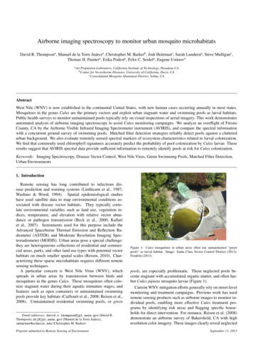
100evaluation. We examined all houses appearing in a fixed geographic area of approximately 2.0 square kilometers outsidethe ground survey area. This subframe was selected to containrange of different commercial and residential areas (Figure 2).We used high resolution satellite images to build a comprehensive list of all pools in the test scene (137 in total). Next, wemarked one pixel of each pool and treat detection scores within10 m (3 pixels) of the mark as successful. This radius was largeenough to capture the largest pools, and small enough that localization errors would not matter to a ground survey team. Wemasked out a canal that transected the subframe, since large water features would be easy to exclude with GIS data in a fullyautomated system.BackgroundPools90Mahalanobis distance β80706050403020100 0.500.511.5Matched filter score α22.52.3. Pool CharacterizationAfter the initial detection step we used reflectance spectrato characterize the condition of each pool. Mosquito colonization of unmaintained pools often coincides with accumulationof spectrally distinctive algae and other organic material. Studies by Reisen et al. (2008) state that larval colonization is associated with lower concentrations of pool chemicals, whichalso lead to algal blooms. We hypothesized that commonlyused spectral water quality indicators, such as measures of algae, chlorophyll and suspended solids, might predict mosquitocolonization. Most previous water quality analyses involve controlled laboratory environments (Han, 1997) or remote sensingof large natural bodies of water (e.g. Kallio et al., 2001; Yacobiet al., 1995; Dekker et al., 2002, and references therein). Residential pools introduce additional complications, such as anoptical path that includes reflection from the pool bottom andthe presence of non-water materials in the AVIRIS pixel. However, pools are physically isolated from each other and permitmany independent trials in a small geographic area.We first considered spectral signatures related to algae.Algae-laden water contains several diagnostic spectral featuresindependent of the presence of other suspended solid material.These features appear in studies based on laboratory measurements (Han, 1997), in situ field measurements (Yacobi et al.,1995), and remote sensing data (Dekker et al., 2002). Algae exhibit low reflectance in the 400 500nm region. There are multiple reflectance peaks caused by local minima in pigment absorption - a strong peak between 550 and 580 nm, and anotherat 650 nm (Dekker et al., 2002). There is a reflectance minimum near 670 due to absorption by chlorophyll. Reflectancesthen increases to a 700 nm NIR peak caused by an interaction ofcell scattering, pigment, and absorption. The chlorophyll-a concentration is a common primary inversion parameter for remotesensing of phytoplankton pigments. It typically involves a ratioof reflectances in the region from 670 720 nm (Kallio et al.,2001). Other ratios are possible; Hoogenboom et al. (1998) estimate these concentrations with the ratio of bands at 715 nmand 667 nm, capturing chlorophyll and pheaophytin pigmentfeatures. We also considered spectral measures of Turbidity,used here as a proxy for Total Suspended Solid matter (Kallioet al., 2001). In general, suspended sediment has been shownto cause an increase in reflectance across the 600-710nm range(Han, 1997). In algae-laden water this feature remains strongest3Figure 3: Matched filter and outlier rejection scores α and β, for each pixel inthe test subframe.βi (x µ(αi ))T Ψ 1 (x µ(αi ))T(5)Large β values indicate outlier pixels. Figure 3 shows an example of α and β values for pixels the test subframe. Most poolpixels were easily separable from the background distribution.In order to make the detection decision one must combinethe α and β scores into a scalar score. This combined scoreis typically a linear combination of αi and βi , but the optimalweighting depends on characteristics of the data. Here we setthe coefficients by injecting synthetic spectra of pools into anurban scene at mixing ratios between 0 and 1, producing αand β scores for both target and background pixels. We thenfit a linear discriminant which best separated the two populations, using a logistic regression mapping onto class labels 1and 0 for the pool and non-pool classes, respectively (Bishop,2006). Other linear discriminants are possible - for example,Foy et al. (2009) use a Support Vector Machine. In practice, wefound performance was insensitive to the precise form of thedecision boundary and any reasonable combination improvedperformance vis a vis matched filters that did not include the βscore.The matched filter algorithm required a representative spectral library. We gathered these target spectra directly from poolsthat were visible in urban AVIRIS scenes. For these tests weformed a target vector t based on the mean spectrum of thepools identified from the MAD survey database. The middlepanel of Figure 2 shows the result, with pixel brightness indicating the strength of the match.We then evaluated true and false detection rates by exhaustively labeling all visible pools in a subframe of the AVIRISoverflight. The MAD database was not suited for this purposebecause it did not include all pools in its geographic region.Therefore it could not identify a false positive; spurious detections within its boundaries could simply have been unrecordedpools. Fortunately even small pools were quite easy to see inthe high-resolution satellite remote sensing data (Google, 2012;Nokia/DigitalGlobe, 2012), so we used this as a standard for4

1at approximately 700 nm, and Kallio et al. (2001) measure turbidity with the reflectance at 710 nm.In this study a logistic regression model (Bishop, 2006) represented the relationship between one or more spectral parameters and the presence of mosquito larvae. It estimated the probability Pθ that a pool harbored Culex larvae based on one or morevariables of interest. For independent variables v {v1 , . . . , vn }and free parameters Θ {θ0 , . . . θn } the model was:1.1 exp[ (θ0 θ1 v1 . . . θn vn )]Fraction of pools detectedPΘ 0.95(6)0.90.850.8Matched Filter (AVIRIS)We report performance from models formed using each ofthe aforementioned spectral attributes. We also fit a multivariatemodel with a wide spectral range, using all channels between400 nm and 2500 nm except the atmospheric H2 O absorptionbands as before. We fit all model coefficients using standardmaximum likelihood methods detailed by Bishop (2006), without regularization terms.We evaluated performance by comparing breeding and nonbreeding classifications against the MAD reference. We estimated classification accuracy rates using Leave One Out CrossValidation (LOOCV) (Dreiseitl & Ohno-Machado, 2002).Specifically, we fit coefficients using all but one data point andthen applied the resulting model to classify the held out datum. We repeated the procedure over the entire dataset andcomputed the expected accuracy rate. This gave an unbiasedestimate of how a similar classifier trained on the entire datasetwould perform on new instances from the population (Kearns& Ron, 1999).0.75NDWI (AVIRIS)NDWI (GeoEye equivalent) 410 3 21010False detection rate 110010Figure 4: Performance comparison for spectral detection methods based onmatched filtering and the Normalized Difference Water Index (NDWI).rate of 10 4 revealed 131 real pools, providing 95% recall withapproximately 7 false alarms per square kilometer. This wascomparable to the accuracy reported by Kim et al. (2011) whouse a combination of color and morphological analysis. Poolsshowed distinctive signatures combining high reflectivity in visible wavelengths with a 850nm water absorption feature. Thismade them relatively simple to detect, and there was no singlepredominant cause of errors. Rare synthetics like plastic roofingmaterials occasionally caused false positives. There was occasionally confusion inside dark shadows, a common challengefor urban remote sensing (Lachérade et al., 2005; Dell’Acquaet al., 2005). Shadows could also prevent detection when overhanging trees or buildings obscured a real pool.3. Results3.1. Pool Detection ResultsWe first evaluated matched filter detection by comparing performance to the Normalized Difference Water Index (NDWI)from McFeeters (1996) and Kim et al. (2011). Their work usesgreen and near infrared bands of satellite data having higherspatial resolution but lower spectral resolution. For an accuratecomparison we spectrally coarsened AVIRIS radiance values tomatch the GeoEye bands (Red: 510-550nm, NIR: 800-910nm).We also considered an NDWI score computed from the highspectral resolution, atmospherically corrected reflectances (Table 1).Both the Matched Filter and NDWI produced scores for every pixel. To detect discrete pools one must threshold this scoreat a level which balances the number of true and false detections. Figure 4 represents this tradeoff with a Receiver Operating Characteristic (ROC) curve (Fawcett, 2004). Desirablecurves (near the upper left) have many true detections and fewfalse positives. We compare NDWI detection strategies withthe matched filter approach, cautioning that our NDWI statistic does not include the additional morphological analysis ofKim et al. (2011) due to the lower spatial resolution. Thematched filter performed better than the NDWI approach using GeoEye-equivalent and AVIRIS spectral resolutions. It detected 122 of 137 pools without false alarms. A false detection3.2. Pool Characterization ResultsThe spectra of breeding and nonbreeding groups separatedvisually into distinct populations. Figure 5a shows the median spectrum from each group, with confidence bars indicating the middle quartiles. Figure 5b shows the first derivativeof the spectrum. The breeding pool data was consistent withall algae chlorophyll signatures noted by Han (1997). A lowerslope in the 400-500nm range may indicate algal absorption. A550nm green peak was present, though it also appeared (somewhat blue-shifted) in clean pools. A concavity in the breedingpool spectra was consistent with a 670nm chlorophyll absorption feature. A relative peak at 700nm appeared in breedingpools and may also be related to chlorophyll (Gitelson, 1992).Finally, the breeding pools also exhibited a shallower slope inthe 500-600nm range.We evaluated each of these spectral attributes for predicting the breeding / nonbreeding distinction. Table 1 showsleave-one-out model prediction accuracies and Kappa statistics(Fielding & Bell, 1997) at the best-performing thresholds. EachRa,b represents the mean reflectance value between wavelengthsa and b (Lunetta et al., 2009). Turbidity performed only slightlybetter than random. The NDWI index correlated somewhat with5

202.5Non breedingBreedingNon breedingBreeding2181.5Derivative of ReflectanceReflectance (%)16141210810.50 0.5 1 1.56 24400450500550600Wavelength (nm)650700 2.5400750450500550600Wavelength (nm)650700750Figure 5: Spectra from pools surveyed by the Consolidated Mosquito Abatement District. 25 Pools from each class are represented. Error bars indicate the medianand middle quartile radiance values for the reflectance spectra (top panel), their first derivative with respect to wavelength (bottom panel).acterization. With spectra expressed as fractional surfacereflectance, the top-performing logistic regression model usingchlorophyll was simply:Table 2: Performance of models formed by multiple spectral attributes, withKappa coefficients and predictive accuracy for the breeding / nonbreeding distinction. The model based on chlorophyll outperformed every combination except for the full spectrum data.CCombinationTurbidity onlyNDWI onlyNDWI, TurbidityChlorophyll, NDWIChlorophyll, TurbidityChlorophyll, NDWI, TurbidityChlorophyll onlyFull ctive � 11 exp( 240 243.3c)forc R685 691R670 677(7)This assumed an even balance of breeding and nonbreedingpools, so widely unbalanced distributions would require appropriate weighting to preserve accurate probability estimates.4. DiscussionThis study demonstrates that airborne imaging spectroscopycan assist WNV vector control. For the task of pool detection,AVIRIS reflectance data provides performance comparable tothe GeoEye studies of Kim et al. (2011), without the high spatial resolution of that instrument. The full spectrum detectionis valuable to find green pools having subtle water absorptionsignatures. After detection, the spectral data is uniquely helpfulfor characterizing pool condition. We find that remotely sensedchlorophyll-a signatures predict mosquito colonization. A bandratio related to chlorophyll-a approaches the predictive powerof a full-spectrum model, classifying colonized and clean poolswith over 94% accuracy for this dataset. Separating detectionand characterization allows both steps to be validated and refined independently. For example, the detection could add morphological or GIS cues, while characterization could incorporate seasonal priors on colonization probabilities.In reality the observed spectrum is affected by the bottom reflectance as well as optical properties of the water (Kim et al.,2010). Residential pools have a wide range of synthetic colorsand materials. Many pool bottoms appear green to the humaneye and can be mistaken for algae in visible images. Spectroscopic data overcomes this problem by revealing the uniquespectral signatures of algal pigmentation and scattering. OurCulex infestation, but the chlorophyll indices achieved betterperformance. The ratio of 685 691 nm and 670 677 nmbands noted in Kallio et al. (2001) had the best cross-validationerror.Table 2 shows prediction accuracy for models formed fromcombinations of multiple variables. The combinations usedthe best-performing band ratios from Table 1. Notably, theturbidity feature bolstered the predictive performance of theNDWI, suggesting that these indicators may be complementary. However, chlorophyll signals alone achieved a far bettercross-validation error rate, outperforming any combination ofmultiple variables with the sole exception of the full-spectrumdata that performed only slightly better. Figure 6 illustrates logistic regression models made from two different pairs of variables. The left and right panels show models formed by pairingNDWI with chlorophyll and turbidity attributes. Each plot indicates probability isocontours at the 5%, 50%, and 95% levels.The populations separated most cleanly along the chlorophyll-afeature.The simplicity and physical interpretability of thechlorophyll-a relationship recommends it for pool char6

Table 1: Definition and predictive accuracy of spectral water quality variables.VariableNDWIChlorophyll-aTurbidityFull spectrumValue(R555 565 R800 900 )/(R555 565 R800 900 )R704 713 /R670 680R699 705 /R670 677R685 691 /R670 677R699 714 /R661 667R674 /R693R704 713 /R675 685R705 714R699 705R705 714 R747 755R705 714 /R747 755[R400 . . . R1206 , R1433 . . . R1732 , R1957 . . . R2500 ]Kappa0.530.740.820.890.770.870.82 0.0 0.00.110.090.92 0.4 0.6 0.60.981Chlorophyll a1.021.04 0.8 0.51.060.5950.50.0.950.0.5050.950.50.050.965 0.40. 0.2050.950.50.050 0.20.940.0.2950.2Breeding0.050.4NDWI0.40Not breeding0.60.Not breedingBreeding0.950.50.050.6 0.80.92Kim et al. (2011)Hoogenboom et al. (1998)Kallio et al. (2001)Kallio et al. (2001)Kallio et al. (2001)Lunetta et al. (2009)Richardson (1996)Kallio et al. (2001)Kallio et al. (2001)Kallio et al. (2001)0.80.8NDWIPredictive .1%59.0%56.4%96.2%00.511.52TurbidityFigure 6: Logistic regression models related spectral attributes to the presence of Culex larvae. Left: A model combining NDWI and chlorophyll attributes.Chlorophyll showed the strongest predictive relationship of all the spectral ratios. Lines indicate probability isocontours at 5%, 50%, and 95% levels. Right: asimilar model using NDWI and Turbidity attributes.7

model uses this to directly estimate the probability of colonization; it averages over pool bottom, surface and volume effects toproduce an expedient result that is readily interpre

Airborne imaging spectroscopy to monitor urban mosquito microhabitats David R. Thompson a, Manuel de la Torre Juarez , Christopher M. Barkerb, Jodi Holemanc, Sarah Lundeena, Steve Mulliganc, Thomas H. Painter a, Erika Podest , Felix C. Seidela, Eugene Ustinov aJet Propulsion Laboratory, California Institute of Technology, Pasadena CA bCenter for Vectorborne Diseases, University of California .