Transcription
The Journal of the Astronautical Sciences (2022) 07-1ORIGINAL ARTICLEDocking Manoeuvre Control for CubeSatsFabrizio Stesina1· Sabrina Corpino1 · Carlo Novara1 · Simone Russo1Accepted: 25 January 2022 / Published online: 3 March 2022 The Author(s) 2022, corrected publication 2022AbstractRendezvous and docking missions of small satellites are opening new scenarios toaccomplish unprecedented in-obit operations. These missions impose to win the newtechnical challenges that enable the possibility to successfully perform complex andsafety–critical manoeuvres. The disturbance forces and torques due to the hostile spaceenvironment, the uncertainties introduced by the onboard technologies and the safetyconstraints and reliability requirements lead to select advanced control systems. Thepaper proposes a control strategy based on Model Predictive Control for trajectory control and Sliding Mode Control for attitude control of the chaser in last meters before thedocking. The control performances are verified in a dedicated simulation environmentin which a non-linear six Degrees of Freedom and coupled dynamics, uncertaintieson sensors and actuators responses are included. A set of 300 Monte Carlo Simulation with this Non-Linear system are carried out, demonstrating the capabilities of theproposed control system to achieve the final docking point with the required accuracy.Keywords Model Predictive Control · Sliding Mode Control · Rendezvous anddocking · Small Satellites1 IntroductionRendezvous and docking (RVD) between spacecraft are very attractive operationswhich enable a large set of space missions. Beyond the spacecraft periodic cargoand crewed mission to ISS, a wide range of relevant missions can be performed such* Fabrizio Stesinafabrizio.stesina@polito.itSabrina Corpinosabrina.corpino@polito.itCarlo Novaracarlo.novara@polito.itSimone Russos266302@studenti.polito.it1Politecnico di Torino, Corso Duca degli Abruzzi 24, 10129 Torino, Italy1Vol:.(1234567890)3
The Journal of the Astronautical Sciences (2022) 69:312–334313as inspection or observation [1], active removal of space debris [2] and not collaborative spacecraft [3], space tugs for refilling on orbit vehicles or move spacecraftfrom lower to high Earth orbit and vice versa [4], and formation flying [5].These missions can be performed or supported by small satellites. CubeSats andnanosatellites might well serve the purpose of inspecting orbiting spacecraft, inthe terms of free-flyers operating in the vicinity of the target for a certain amountof time, while observing the target with suitable sensing equipment. In September2019, the 3U CubeSat named Seeker was launched by NASA and operated aroundCygnus, taking images of the vehicle and performing a set of manoeuvres (such astarget tracking and station-keeping) [6]. Other studies on the inspection missions byCubeSat have been carried out also by the European Space Agency (ESA) [7] and[8]. The Ecole Polytechnique Federal de Lausanne is leading the CleanSpace Oneproject with the objective of removing the 1U Swiss Cube satellite from orbit usinga CubeSat [9]. The CleanSpace One mission will also demonstrate in orbit technologies needed for other ADR missions. In [10], the authors show a set of architectures for CubeSat in different scenarios on a complexity spectrum of uncooperativeto cooperative. In [11], the authors provide the mission concepts and preliminarysystem design of a CubeSat devoted to the inspection of the cis-lunar space station,showing the advantages of the external inspection mode with a small satellite thatfly-around the station and the challenges in terms of required onboard technologyand control strategies.Adopting small satellites for rendezvous missions is challenging because of thereduced dimensions and the available technologies, that are achieving the requiredlevel of maturity only in the last years. In this sense, In Orbit Demonstration missions are planned and advanced studies are conducted to improve the level ofreadiness for small satellite technology. NASA, ESA, and other organisations andcompanies are also working on CubeSat missions for demonstrating capabilitiesrelated to formation flight and proximity operations, which have relevance for thepurpose of inspecting vehicles in orbit (e.g. NanoAce 3U CubeSat flown in 2017[12], GOM-x-4B 6U CubeSat flown in 2018 [13], CubeSat Proximity OperationsDemonstrator (CPOD) to be launched in 2021 [14] Dedicated studies are conductedon critical technologies of the mating phase, the relative navigation and the docking mechanism. A vision-based navigation strategy based on advanced images processing algorithms are reported in [15], while [16] proposes a vision-based poseestimation combined with robust Higher-Order Sliding Mode (HOSM) controllersis explored. Branz et al. [17] propose miniaturized docking mechanisms based onthe probe–drogue configuration using a minimum number of actuations and movingparts.All the rendezvous and docking missions require that a critical set of manoeuvresallow the Chaser spacecraft to operate in proximity to the Target spacecraft, oftenup to the docking that ends when the two spacecraft are kept in touch in the matingpoint. The last meters before the mating are very critical because the margin of erroris reduced. One way to improve the confidence level in the success of the dockingphase is to adopt an effective strategy to control the relative attitude and distance13
314The Journal of the Astronautical Sciences (2022) 69:312–334between Target and Chaser. In [18], the authors study controllers based on LinearQuadratic Regulator (LQR) and Proportional Derivative (PD) Control, verifying theperformance and robustness of the solutions without considering other parameterssuch as time and control effort. In [19], the authors use the same control laws of[18] and present a comparative analysis between different guidance trajectories forimportant parameters such as time, fuel consumption, minimum absolute distance,and the maximum radial distance from the target without highlighting the optimalityof the results. Adaptive control laws for spacecraft rendezvous and docking undermeasurement uncertainty, such as aggregation of sensor calibration parameters, systematic bias, or some stochastic disturbances, are proposed in [20]. In [21], authorsshow an optimized state dependent Model Predictive Control (MPC) that integratesa pulse width pulse frequency modulation model: the results highlight a good accuracy for the reaching the final state minimizing the control efforts and approachingtime. Ventura at al. [22] proposes a guidance scheme for autonomous docking wherethe trajectory components of the controlled spacecraft are imposed by using polynomial functions determined through optimization processes. From the manoeuvre’sstrategies point of view, the authors in [23] give a complete overview of the manoeuvre and control capabilities for the capture of a non-rotating and of a rotating target,using a MPC but limiting the study to planar manoeuvres. One of the key points forMPC controller is the ability to handle constraints on state vector and control vectors: [24] presents a strategy for spacecraft rendezvous control based on linear quadratic MPC with dynamically reconfigurable constraints. In [25], authors present aMPC focused on the tracking based capability for a chaser involved in the capture ofa non-cooperative spacecraft discussing advantages and criticalities of this approachthrough analysis of the time and the control efforts required to achieve the matingpoint. Mammarella et al. [26] propose and validate on a test-bench a sampling-basedstochastic model predictive control (SMPC) algorithm for discrete-time linear systems subject to both parametric uncertainties and additive disturbances.In the small satellite’s context, few papers address the control problem for thefinal approach and mating phases of rendezvous. Bowen et al. [27] presents thedetermination and control strategy for CPOD mission, but no further details areprovided on the adopted techniques. Pirat et al. [28] present an H-infinity controller taking care the robust stability and performance through mu-synthesis.Stesina in [29] reports a solution based on a tracking MPC without including theattitude control.The present paper presents a control strategy that maintain de-coupled the rotational and translational dynamics based on the MPC and Sliding Mode Control techniques, in order to optimize the final position and attitude of the chaser limiting thefuel consumption and the time to perform the capture. After the problem definitionin Sect. 2, the design of the controller and the tuning of its parameters is proposed inSect. 3. Section 4 reports and discusses the results of simulations for different initialconditions and uncertainties on the spacecraft parameters. Section 5 concludes thepaper with final remarks and the future perspectives of the work.13
The Journal of the Astronautical Sciences (2022) 69:312–3343152 Problem formulationThe objective is the control of the relative position and attitude between the targetand chaser. The problem formulation is based on the definition of the adopted reference frames and assumptions on the motion conditions and the spacecraft features.2.1 Reference framesFour reference frames are defined in order to formulate the problem (Fig. 1). The ECEF (Earth-centered Earth-fixed) frame (RI ) is considered a quasi-inertialframe for the mission and it has origin O I in the centre of the Earth, x I in theequatorial plane, pointing toward the mean of the vernal equinox; zI is normalto the equatorial plane and pointing north, yI is in the equatorial plane, such that zI xI yI. The Spacecraft Local Orbital frame ( Ro ) has its origin Oo in the centre ofmass (CoM) of the spacecraft; xo is defined such that xo yo zo (xo is in thedirection of the orbital velocity vector but not necessarily aligned with it), yois in the opposite direction of the angular momentum vector of the orbit and zo is radial from the spacecraft CoM to the centre of the Earth. In this paper,both the Target Local Orbital Rotg (Oot, xot, yot, zot) frame and the ChaserLocal Orbital frame Roch(Ooch, xoch, yoch, zoch) should be taken into account.Since distance(OotOoc) distance (OotOi) and distance(OotOch) distance (OocOi), we can assume that Roc Rot Ro.Fig. 1 Schematic of the reference frames13
316The Journal of the Astronautical Sciences (2022) 69:312–334 The Target Body frame ( Rt ) has origin O t in the Target centre of mass,the directions of the axes are along the main inertia axes of the Target and zt xt yt forming a right-handed system. The Chaser Body frame ( Rc ) has origin O c in the Chaser centre of mass,the directions of the axes are along the main inertia axes of the Chaser and zc xc yc forming a right-handed system.2.2 AssumptionsThe problem formation is based on a set of assumptions on the motion conditions:Assumption 1 (Last Hold Point orbit conditions) The control starts in the finalhold point (HP) at 50-meters of distance between chaser and target and Chasermechanism is already aligned with the docking port when moves from the HP.This assumption allows us to consider guidance strategies based on straight-lineapproaches. The achievement of this final hold point depends on the previous mission phases; an example is provided in [8].Assumption 2 (Last hold Point attitude conditions) The target reaches any orientation in space but it maintains this orientation for the entire duration of the manoeuvre. This allows defining a fixed desired attitude that the chaser has in the HP andshall maintain for the entire duration of the manoeuvres. Other assumptions derivefrom the spacecraft configuration.Assumption 3 (Chaser and Target mass properties) Target and chaser are 12U CubeSats (20 cm 20 cm 30 cm) whose mass (m) is 20 kg and the inertia (expressedin the respective body frame) is diagonal I cx Itx 0.133, Icy Ity 0.216, I cz Itz 0.216. In general, the two CubeSats should have a different architecture and differentonboard instruments because the Target should only maintain the attitude withoutorbit control, while the chaser shall determine and change its orbit and needs of specific sensors and actuators dedicated to this purpose. However, the perfect similarity of the two spacecraft can be justified by reliable considerations: both the CubeSats have the complete attitude and orbit control systems enabling the possibility toexchange the role of target and chaser in case of anomaly for the orbit control of theregular chaser.Assumption 4 (Location of the docking port and docking mechanism) Due to thesmall dimensions of the satellites and considering a fixed distance of the dockingport with respect to Oc along Xc axis and fixed distance of the docking mechanismwith respect to Ot along Xt axis, it is assumed that the docking port and the dockingmechanism are located in coincidence of Ot and Oc, respectively.Assumption 5 (Rotational Dynamics of Chaser and Target) The Target body axes arealigned with the orbital frame (i.e. Rt Ro). It means that if the Chaser controller is13
The Journal of the Astronautical Sciences (2022) 69:312–334317able to control the attitude reaching and maintaining the Chaser body axes alignedwith the orbital frame (i.e. Rc Ro), Target and Chaser have the attitude.3 Control designThe goal of the controller is to reach the soft docking performance described inTable 1 guaranteeing efficiency and safety conditions. More specifically, the goalis to control the Chaser attitude and angular velocity and the relative position andvelocity between the Chaser and Target, according to the strategies defined for anyphase (see Sect. 4.1). The controlled state variables are: the attitude ( qc) and theangular velocity (ωoc) between the Chaser Body Frame (Rc) and orbital frame (Ro)and the relative position (x,y,z) and velocity ( Vx, Vy, Vz) between the Chaser CoM (Oc) and the Target CoM (Ot).The control design and assessment phases are articulated in two steps: the designis based on a linearized spacecraft model, while the verification is led through amore complex and nonlinear model of rotational and translational dynamics of thechaser including disturbances and uncertainties.The control design foresees the de-coupling of the rotational and translationaldynamics, that allows us to select different techniques to control the attitude and therelative trajectory between Chaser and Target.A Model Predictive Controller (MPC) is designed for the control of the Chasertrajectory. The advantages of this technique for the rendezvous and docking problemare: 1) the possibility to constrain the input, the state and output imposing boundaries whose violation is prevented and 2) the capability to jointly define an optimalguidance strategy and the feedback command allowing the spacecraft to follow thisstrategy, 3) constraints or penalties on fuel consumption, time to capture and safetyconditions of the manoeuvre can be introduced. 4) MPC can drive some variablesto their optimal set points (i.e., the relative position can be optimized to meet thesoft docking requirements) while others can be held within imposed ranges (i.e. thevelocity can be regulated with specific profiles). The prediction of the future statesleads to the definition of an optimal trajectory. For the MPC design in this research,a reference tracking optimization criterion is introduced in order to assign a higherimportance to the capability of the controller to track the desired values.Table 1 Final requirementsRequiredPerformanceApproach velocity [m/s] 0.05Lateral alignment [m] 0.02Lateral velocity [m/s] 0.02Angular misalignment [deg] 1Angular rate [deg/s] 0.0513
318The Journal of the Astronautical Sciences (2022) 69:312–334A Sliding Mode Controller is designed for the control of the Chaser attitude. Theadvantages of this approach applied to the presented rendezvous and docking problem are: 1) capability to efficiently deal with nonlinear dynamics and 2) robustnessversus modelling uncertainties.3.1 Trajectory control3.1.1 Model predictive control lawIn this section, we present a general formulation of Model Predictive Control(MPC), suitable for nonlinear and linear systems [29].Consider a dynamic system described by the following state equation:ẋ f (x, u)(1)where x ℝnx is the state, u ℝnu is the command input and f ℝnx nu ℝnx is afunction characterizing the system dynamics. Assume that the state is measured inreal-time, with a sampling time Ts, according to x(tk ), tk Ts k, k 0, 1, Suppose that the system state x is required to track a desired reference signal r .The state and input variables may be subject to constraints and it may be of interestto have a suitable trade-off between performance and command effort. MPC is asuitable approach to solve such a control problem [30].MPC is based on two key operations: prediction and optimization. At each timet tk , the system state is predicted over the time interval [t, t Tp ], where Tp Ts iscalled the prediction horizon. The prediction is obtained by integration of the system Eq. (1). For any 𝜏 [t, t Tp ], the predicted state ̂x(𝜏) is a function of the “initial” state x(t) and the input signal:̂x(𝜏) ̂x(𝜏, x(t), u(t 𝜏))where u(t 𝜏) denotes the input signal in the interval [t, 𝜏]. The basic idea of MPCis to look, at each time t tk , for an input signal u (t 𝜏) such that the prediction̂x(𝜏, x(t), u (t 𝜏)) has the desired behavior in the time interval [t, t Tp ]. The concept of desired behavior is formalized by defining the objective function J u(t t Tp ) t Tp t ‖̃xp (𝜏)‖2Q ‖u(𝜏)‖2R d𝜏 ‖̃xp (t Tp )‖2Px(𝜏) is the predicted tracking error, r(𝜏) ℝnx is the referencewhere x̃ p (𝜏) r(𝜏) to track and ‖ ‖ is a weighted vector norm. For a generic vector x and a positivedefinite weight matrix Q, this norm is defined as follows:‖x‖2Q x Qx.In most cases, diagonal weight matrices are used since the non-diagonal terms are ingeneral difficult to manage/interpret and their utilization usually does not yield relevantadvantages.13
The Journal of the Astronautical Sciences (2022) 69:312–334319u (t t Tp ) is chosen as one minimizing the objective function( The input signal)J u(t t Tp ) . In particular, at each time t tk, for 𝜏 [t, t Tp ], the following optimization problem is solved:()u (t t Tp ) argmin J u(t t Tp )u( )( subject to)̇ x(𝜏) f x(𝜏), u(𝜏) , x(t) x(t) x(𝜏) Xc , u(𝜏) Uc(2)where 0 Ts Tc Tp. The fist constraint in this problem ensures that the predicted state is consistent with the system Eq. (1). The set Xc accounts for possibleconstraints that may hold for the state trajectory (e.g., obstacles, barriers, etc.). Theset Uc accounts for input constraints (e.g., input saturation).The MPC feedback command is obtained by solving the optimization problem ateach sampling time t tk, according to a so-called receding horizon strategy: At time t tk:– compute u (t t Tp ) by solving (2);– apply to the system only the first input value: u(𝜏) u (t tk ) and keep itconstant for 𝜏 [tk , tk 1 ]. Repeat the two steps above for t tk 1 , tk 2 , Note that the optimization problem in Eqs. (2) is in general non-convex. Moreover,the decision variable u( ) is a signal and optimizing a function with respect to a signal is in general a difficult task. To overcome this problem, a suitable parametrizationof the input signal u is taken. In particular, the prediction interval [t, t Tp ] is dividedinto sub-intervals [t 𝜏i , t 𝜏i 1 ] [t, t Tp ], i {1, 2, , nI 1}, where the 𝜏i’s arecalled the nodes. Then, u is assumed constant on each sub-interval, so that the optimization problem reduces to a finite-dimension problem, which is solved using an efficient numerical optimization algorithm.3.1.2 MPC for trajectory controlThe assumptions of small initial relative position and short maneuver time allow us touse the well-known Hill–Clohessy–Wiltshire model, describing the motion of a spacecraft (called the Chaser) relative to a nominal point traveling in a circular orbit (calledthe Target orbit). This model is described by the following equations:ẍ c 2Ωż c ÿ c Ω2 yc z̈ c 2Ωẋ c FcxmcFcymcF3Ω2 zc mczc(3)where xc, y c, zc are the relative Chaser positions, mc is its mass, Ω is the angular frequencyof the Target orbit, and Fcx, Fcy and Fcz are the external forces applied to the Chaser.13
320The Journal of the Astronautical Sciences (2022) 69:312–334Equations (3) can be represented in the form of the state equation (1) as follows:ẋ Ax Buwhere x ( xc, yc, zc, ẋ c, ẏ c , ż c) is the state vector, constituted by the three components of the Chaser position and velocity with respect to Rt , u (Fcx,Fcy,Fcz ) is theforce vector, and 0 0 0A 0 0 00000 Ω3Ω20 10 00 00 00 00 2Ω20100000 0 1 2Ω2 0 0 B 0 0 0 0 0 0 0 0 0 10 0 mc 0 m1 0 c0 0 m1 cThe MPC control law is obtained by solving, at each sampling time, theoptimization problem in Eqs. (2), according to the receding horizon strategydescribed in the above section. In the optimization problem, the model function is f (x, u) Ax Bu . The input constraint set Uc is defined by the followinginequalities: Fcmax u Fcmaxwhere Fcmax is the vector of the maximum thruster forces and the inequalities areelement-wise. The state constraints depend on the approach corridor represented bythe cone originated from the mating point and with a half cone angle of 𝛿 . Considering the assumptions made in Sect. 2, the cone is univocally defined for the straightline maneuver, and it is generated from the docking point and it is centered in thedocking axis, the Xc axis. Therefore, the state constraint set is defined by the following inequalities:axy xc sin(𝜑 𝛿) yc cos(𝜑 𝛿) 1bxy xc sin(𝜑 𝛿) yc cos(𝜑 𝛿) 1axz zc sin(𝜃 𝛿) xc cos(𝜃 𝛿) 1bxz zc sin(𝜃 𝛿) xc cos(𝜃 𝛿) 1(4)where axy, axz , bxy and bxz represent the corridor limits, and 𝜑 and 𝜃 are the anglesbetween the docking axis and Rt axes. These angles are assumed constant for theentire prediction horizon. Figure 2 refers to the specific case (considered in thispaper) of V-bar approach, where phi and theta are equal to 180 deg.The MPC weight matrices Q and R (defined as Q diag(Q11, Q22, Q33,Q44,Q55,Q66), R diag(R11,R22,R33)) are tuned to satisfy the requirements in Table 1.Note that the set Uc is convex. If the chaser initial conditions are inside the cone,also the set Xc is convex. Hence, with f (x, u) Ax Bu, the optimization problemof Eqs. (2) becomes convex, which implies that every local solution of this problem is a global solution. Another implication is that convex algorithms can be usedfor its solution, which are characterized by a high numerical efficiency and strong13
The Journal of the Astronautical Sciences (2022) 69:312–334(a)321(b)Fig. 2 Safety cone definitionconvergence properties. In this paper, an algorithm based on quadratic programmingis adopted, suitably modified for the considered application.As discussed in the above section, it is convenient to parametrize the input signal by dividing the prediction interval into sub-intervals and assuming u constanton each sub-interval. In this paper, a single sub-interval is assumed for simplicity( 𝜏1 0, 𝜏2 Tp ). Larger numbers of sub-intervals were considered in preliminarysimulation sessions, but no relevant improvements were observed.3.2 Attitude control design3.2.1 Sliding mode controlIn this section, we present a standard formulation of Sliding Mode Control(SMC), that is particularly suitable for mechanical systems.Consider a dynamic system described by the following state equations:ṗ vv̇ f (x) g(x)u(5)where p, v ℝnp, x (p, v) ℝnx is the state and u ℝnu is the command input;f ℝnx ℝnp and g ℝnx ℝnp are two functions characterizing the systemdynamics. Note that many mechanical systems can be written in the form (5), with pbeing a position vector and v a velocity vector.Suppose that the system state x (p, v) is required to track a desired referencesignal r (pr , vr ). SMC is a suitable approach to solve this tracking problem.SMC is based on the concept of sliding surface, that is a surface S(t) in the statedomain, defined as13
322The Journal of the Astronautical Sciences (2022) 69:312–334S(t) {x ℝnx 𝐬(x, t) 0}𝐬(x, t) ṽ k2 p̃where the tracking errors p̃ pr p and ṽ vr v have been introduced, andk2 0. A fundamental property of S(t) is that, if the motion of the system stateoccurs on this surface, then the tracking errors converge to zero [29].Based on the sliding surface, the following SMC law is defined:u )1 (v̇ r f (x) k2 ṽ k1 sign(𝐬(x, t))g(x)(6)where k1 0. It can be proven that this law is able to bring the system state to thesliding surface and, once there, to keep the state on it [29]. In summary, with thislaw, the following properties hold: S(t) is globally attractive: x(t) S(t) in finite time. S(t)is an invariant set: x(𝜏) S(𝜏) x(t) S(t), t 𝜏 . On S(t) the tracking errors converge to 0: p̃ (t), ṽ (t) 0 as t .It must be noted that the term with the sign in the control law may cause a phenomenon called chattering (high frequency oscillations around the sliding surface).To avoid this problem, a sigmoid function like the hyperbolic tangent can be usedinstead: tanh(𝜂𝐬) sign(𝐬), where 𝜂 is a design parameter determining the sigmoidslope.3.2.2 Sliding mode controller for attitude controlConsidering the Assumption 5, it is possible to design the attitude control using theabsolute rotational dynamics of the Chaser, as in [25], instead the relative dynamics Target/Chaser. A standard model is adopted for the chaser attitude motion. Inparticular, the attitude state equations are obtained using the quaternion kinematicequation and the Euler dynamic equation:𝔮̇ 21 Q𝝎𝝎̇ J 1 𝝎 J𝝎 J 1 𝝎(7)where 𝔮 is the chaser quaternion (rotation from the ECEF to the Chaser Bodyframe), 𝜔 is the chaser angular speed vector, J is the chaser inertia matrix, denotesthe cross product and q1 qQ 0q 3 q2 q2 q3q0q1 q3 q2 . q1 q0 The goal is to have the state vector x (𝔮, 𝜔) tracking a reference vector (𝔮r , 𝜔r ).In order to define a proper SMC law accomplishing this task, we define the angular velocity tracking error as 𝜔 𝜔r 𝜔 and the quaternion tracking error as13
The Journal of the Astronautical Sciences (2022) 69:312–334323 𝔮 𝔮 𝔮r , where 𝔮 is the conjugate of 𝔮 and denotes the quaternion product. Asuitable sliding surface function is 𝐬(x, t) 𝜔 k2 q̃ where q̃ is the imaginary part of 𝔮. The SMC law for the system (7) is given byu( us k1 J tanh(𝜂𝐬) )) q̃ 0 𝜔 ̃q (𝜔r 𝜔) 𝜔 J𝜔us J 𝜔̇ r (k22 where q0 is the real part of 𝔮. See [30] for a detailed derivation of this control law.4 Numerical results4.1 Simulation architectureThe designed controllers are verified using a detailed model and a simulationarchitecture built in the Matlab/Simulink environment (Fig. 3). This architectureincludes models for disturbance torques (i.e. all the torques due to aerodynamicdrag, the solar pressure, gravitational gradient, residual magnetic dipole, and thesloshing of the fuel in the tank) and the disturbance force due to the aerodynamics.The emulation of the attitude and position sensing and estimation is obtained fromFig. 3 Simulation architecture13
324Table 2 Chaser featuresTable 3 Chaser initialconditionsThe Journal of the Astronautical Sciences (2022) 69:312–334ParameterValueUncertaintiesDiag [ Ichx , Ichy , Ichz][0.08;0.16;0.216]kg m2 10%mch Max ( Fcx , Fcy , Fcz ) Max ( Tcx , Tcy , Tcz ) 20 kg alueUncertainties𝜔cx , 𝜔cy , 𝜔cz[0;0;0]rad s 0.2 rad/sq0 , q1 , q2 , q3[1;0;0;0] 10%xc0,yc0,zc0[ 50;0;0] m 2.5 mẋ c0 , ẏ c0 , ż c0[0;0;0] m/s 0.2 m/sthe simulated values (output of the Dynamics and Kinematics Blocks), added byrandom values in the range of 5%. The desired attitude for the Chaser is the current attitude of the Target, while the desired position is the final position. The attitude control actuators consists in the model of three reaction wheels installed alongthe main body axes of the satellite, and the thruster emulation consists of the thrustvalue saturation at the maximum value and an uncertainty of the 5% on the alignment of the thrusters with respect to the chaser axes expressed by the frame Rc.Moreover, the rotational and the translational dynamics of the Chaser are coupled inthe simulation environment, while the controllers for the attitude and the controllerfor the relative position are designed independently.4.2 Cubesat constraints and initial conditionsIn the simulation sessions, the parameters representative of a CubeSat are reportedin Table 2: the inertia matrix is diagonal and the mass is compliant with a 12U andan uncertainties of the 10% is added for both the parameters. The maximum controlled forces and torques are limited by the small satellite technology, i.e., the maximum thrust of a miniaturized propulsion system, that guarantees a 3DoF control,and the maximum torque generated by a set of reaction wheels.Table 3 reports the initial conditions with uncertainties angular velocity and attitude, and relative velocity and position.The satellites travel in a circular orbit with an altitude of 500 km. The controllerssampling time is 0.1 s.Upper and lower bounds are referred to input values, according to the physicallimitations of the propulsion system: the thrusters are able to provide a maximumforce equal to 0.035 N. Since the internal model considered in the MPC formula
reduced dimensions and the available technologies, that are achieving the required level of maturity only in the last years. In this sense, In Orbit Demonstration mis- . (e.g. NanoAce 3U CubeSat own in 2017 [12], GOM-x-4B 6U CubeSat own in 2018 [13], CubeSat Proximity Operations Demonstrator (CPOD) to be launched in 2021 [14] Dedicated .