WIXLIB

and where active adjustments in reserve supply are not needed to implement policy. 2 It is alsoconsistent with the Federal Reserve’s longstanding plan to operate with a balance sheet that is nolarger than necessary for efficient and effective policy implementation. 3We also discuss how the Federal Reserve’s decision on reserve levels in October 2019 can beinterpreted within our framework. Our analysis focuses on the federal funds market, since theFederal Open Market Committee (FOMC) establishes the stance of policy by setting a targetrange for the federal funds rate. As such, we do not attempt to present a complete account ofdynamics across all money markets.Section 5 broadens the consideration of effectiveness to money markets in general. We examinethe operating regime’s ability to provide control over short-term money market rates, asmeasured both by dispersion across these rates and by the pass-through of administered rates tomarket rates. We find that, so far, the evidence suggests a high degree of effectiveness for theFederal Reserve’s current regime.Finally, considering the broader context of the entire financial system, we argue that financialstability concerns may make it socially efficient for the central bank to supply ample reservesrather than make reserves scarce. In particular, an important contrast between implementationmechanisms with ample reserves and the pre-crisis mechanism of adjusting reserve supply tochange the scarcity value of reserves is that a regime operating mainly through adjustments inadministered rates can exert influence on money market rates even after large reserve injectionssuch as those resulting from central banks’ responses to the crisis.2. A Simple Model of Reserve Demand and Interest RatesFor many central banks, the policy rate is the rate that banks pay to borrow reserves overnight.Thus a key factor in discussing monetary policy implementation is the relationship between thelevel of reserves and the overnight interest rate: the aggregate demand curve for reserves. Theshape of the demand curve varies across different theoretical models, and our framework isflexible enough to allow a wide variety of shapes.To motivate the existence of the demand curve and reasonable assumptions on its shape, a goodstarting point is Poole (1968). In this model, banks must hold reserves overnight to meet reserverequirements, but face random payment shocks during the day that can drain their reserves.Banks pay a high penalty rate for failing to meet reserve requirements, and earn a lower or zerointerest rate on reserve balances in excess of requirements. The lower a bank’s reserve holdingsat the beginning of the day, the greater risk it faces of paying a penalty and the more it is willingto pay to borrow reserves as a buffer against payment shocks. The same relationship holds forbanks in the aggregate. Thus, at lower aggregate levels of reserves, market interest rates increaseSee “Statement Regarding Monetary Policy Implementation and Balance Sheet wsevents/pressreleases/monetary20190130c.htm.3See “Policy Normalization Principles and Plans,” September 2014, available ory.htm.24

strongly with decreases in the supply of reserves – a relationship that the central bank can use toinfluence market rates, as we will see later in the paper. At sufficiently high levels of reserves,the demand curve becomes flat at an interest rate equal to the rate paid on excess reserves, andmarket interest rates become unresponsive to reserve supply, but still respond to changes in theadministered rate on excess reserves.The standard model nicely describes the implementation framework used by many central bankspre-crisis, including the Federal Reserve. Before September 2008, the Federal Reserve would seta target for the effective federal funds rate above the interest rate on excess reserves, which waszero at the time. 4 Therefore, the target was on the negatively sloped part of the aggregate demandcurve. The Federal Reserve would supply the appropriate amount of reserves to intersect thedemand curve at the policy target. The amount of total reserves supplied by the Federal Reserveto the banking sector was very small, just under 9.5 billion on average in 2006. Excess reserveswere approximately 1.7 billion. Since banks held reserves primarily to meet reserverequirements, the aggregate demand curve was relatively easy to forecast. As well, the FederalReserve could reasonably anticipate changes in the aggregate supply of reserves that resultedfrom changes in the central bank’s other liabilities, such as currency in circulation. 5 As a result,by conducting daily open market operations to offset changes in aggregate supply and demandfor reserves, the Federal Reserve could hit its policy target.In the United States and many other countries, reserve demand and the functioning of theinterbank market changed after the financial crisis in at least three important ways. First, changesin liquidity supervision and regulations and bank risk management practices increased thedemand for high-quality liquid assets (HQLA), including reserves. Second, reserve demandbecame more uncertain, at least from the central bank’s perspective. Banks can choose how toallocate their HQLA between reserves and government securities, so demand is no longer a staticfunction of regulatory parameters. In addition, even without regulatory changes, the crisis mayhave changed reserve demand by influencing banks’ risk appetites – but this source of demandcan change over time and is not easily observable by the central bank. Third, stricter regulationson banks’ leverage ratios and balance sheet expansion resulted in increased marginal tradingcosts in the interbank market, 6 as did other changes in regulations and risk appetite that indirectlyincreased banks’ perceived cost of trading.We extend the standard model to reflect these post-crisis changes. The extension generatesseveral important findings. First, the level of reserves needed to implement any given marketinterest rate is higher because reserve demand is higher. Second, uncertainty about reservedemand leads to uncertainty about the market interest rate that will be associated with any givenaggregate level of reserves, but the effect is smaller at higher levels of reserves, where thedemand curve is flatter. Third, frictions in the interbank market mean that reserves are notThe Financial Services Regulatory Relief Act of 2006 authorized the Federal Reserve Banks to pay interest onbalances held by or on behalf of depository institutions at Reserve Banks, subject to regulations of the Board ofGovernors, effective October 1, 2011. The effective date of this authority was advanced to October 1, 2008, by theEmergency Economic Stabilization Act of 2008.5Footnote: This ability, in part, reflected policies that limited the variability of certain Federal Reserve accounts.6Kim, Martin and Nosal (forthcoming) study the effect of such regulations on the interbank market.45

always efficiently distributed, in the sense that banks that have a low marginal value of reserveswill not necessarily lend to other banks that have a higher marginal value of reserves. Fourth, atrelatively high levels of reserves, the demand curve may have a region with a gentle slope, wherechanges in reserve supply lead to small – but non-zero – changes in market rates.We emphasize that our model makes significant simplifying assumptions for clarity ofexposition. For example, it focuses on a funding market for similar banks and does not capturedifferences among banks. Nor does the model describe non-bank borrowers, which are importantparticipants in U.S. money markets but whose costs and constraints often differ from those ofbanks. Thus, although the model is useful for understanding control of the federal funds rate –the policy rate in the U.S. – it does not seek to describe the full range of real-world moneymarket dynamics.The remainder of this section provides technical details on the model’s predictions.2.1. Poole (1968) Reserve Demand ModelA large literature on monetary policy implementation uses some variant of Poole (1968). 7 Thissection provides a sketch of the Poole (1968) or standard model. The model assumes that banksdemand reserves to meet their regulatory reserve requirements. The central bank provides morethan enough reserves to meet these requirements. In other words, aggregate excess reserves – thedifference between total reserves and required reserves – are strictly positive.Banks can adjust their reserve holdings in an interbank market which, for the time being, isassumed to be competitive and frictionless. After the interbank market closes, banks receive apayment shock that reallocates reserves among them. If a bank’s payment shock is sufficientlynegative, its reserve holdings will fall below what is required – it will have negative excessreserves. In this situation, the bank must borrow reserves from the central bank at a penalty rate,𝑟𝑟𝑝𝑝 , so that its excess reserves are at least zero. (The value of 𝑟𝑟𝑝𝑝 includes both the explicit ratecharged for borrowing reserves as well as any non-pecuniary stigma associated with discountwindow borrowing.) If the payment shock implies that a bank ends up with positive excessreserves, the central bank pays interest on those reserves, IOR. IOR is strictly less than 𝑟𝑟𝑝𝑝 andcould be equal to zero.If payment shocks are uniformly distributed around zero, then a bank’s demand curve forreserves is described by Figure 1, above (see Ennis and Keister, 2008, for a formal derivation).The demand curve is the locus of indifference points for the bank. Specifically, a bank isindifferent between borrowing and lending a marginal unit of reserves at each combination ofinterest rate and reserve holdings along the demand curve.Some recent work has used other types of model such as search and bargaining or preferred habitat, in contrast toperfect competition in Poole (1968). See for example Afonso and Lagos (2015), Afonso, Armenter, and Lester(2019), Armenter and Lester (2017), Schulhofer-Wohl and Clouse (2018), Kim, Martin and Nosal (forthcoming),and Chen, Clouse, Ihrig, and Klee (2016). Still, in some of these works, demand for reserves originates fromrequired reserves and timing of shocks that are broadly consistent with Poole (1968).76

After the payment shock, the marginal value of reserves to the bank is equal to the penalty rate 𝑟𝑟𝑝𝑝if the bank has negative excess reserves, and is equal to IOR if the bank has positive excessreserves. Before the payment shock, the bank’s willingness to pay for reserves is the expectedmarginal value. Therefore, if a bank’s excess reserves are so low that it always ends withnegative excess reserves after the payments shock, the bank is willing to borrow reserves in theinterbank market at rates up to the penalty rate, 𝑟𝑟𝑝𝑝 . A bank with higher excess reserves has apositive probability that its excess reserves are positive following the payment shock, so itswillingness to pay for an additional dollar of reserves is below 𝑟𝑟𝑝𝑝 . Finally, if a bank’s excessreserves are so high that it always holds positive excess reserves following any payment shock,then the bank is indifferent between borrowing and lending reserves at IOR. 8 Hence, the bank’sdemand curve for reserves has a (weakly) negative slope and lies between IOR and 𝑟𝑟𝑝𝑝 , asillustrated in Figure 1.The equilibrium interbank rate is determined by equalizing aggregate demand and aggregatesupply. 9 The aggregate demand curve for reserves is simply the horizontal summation of theindividual banks’ demand curves; if banks are identical, the shape of the aggregate demand curveis identical to the individual demand curve. The central bank supplies an exogenous amount ofreserves to the banking sector. A vertical line in the interest rate-reserve space represents theaggregate supply of reserves. Figure 2 illustrates two different aggregate supply curves, 𝑆𝑆1 and𝑆𝑆2 . If the aggregate supply of reserves is 𝑆𝑆1, then the interbank rate, 𝑟𝑟𝑟𝑟1, exceeds IOR; if theaggregate supply is 𝑆𝑆2 , then the interbank rate, 𝑟𝑟𝑟𝑟2, equals IOR.We abstract from risk premia for simplicity.In addition, the equilibrium interbank rate equalizes the aggregate demand for loans in the interbank market withthe aggregate supply of loans in that market. This is the case because a bank’s demand for interbank loans equals thedifference between its reserves when the market opens and the quantity of reserves it demands; thus, the aggregatedemand for interbank loans equals the aggregate supply of interbank loans if and only if the aggregate demand forreserves equals the aggregate supply of reserves.897

Figure 2: Equilibrium in the Poole Model.In the standard model, equilibrium in the interbank market is characterized by all banks havingthe same marginal value of excess reserves when the interbank market closes, independent of theinitial distribution of reserves across banks. This common marginal value of excess reserves isthe interbank rate. If the interbank rate exceeds IOR, then assuming that banks have identicalpreferences, all banks must have the same amount of excess reserves when the interbank marketcloses. Hence, if the aggregate supply of reserves is on the steep part of the demand curve, banksholding more than the average amount of excess reserves before the market opens lend in theinterbank market and those holding less than the average amount borrow in the interbank market.However, if the interbank rate equals IOR, all we can say is that all banks will be on the flat partof the individual demand curve; there would be no incentive for borrowing or lending even ifsome banks were further to the right on the flat part of the curve than others.Finally, the interbank market can be replaced with a more general funding market with non-banklenders, and the demand curve for reserves in the standard model remains the same whethertrading occurs in an interbank market or in some other funding market. 102.2. Post-crisis developmentsIn this subsection, we first discuss the impact of liquidity regulation on the demand for reserves.Then we consider how other post-crisis regulatory changes have increased the regulatory costs ofexpanding a bank’s balance sheet and trading in money markets.10See, for example Kim, Martin and Nosal (forthcoming).8

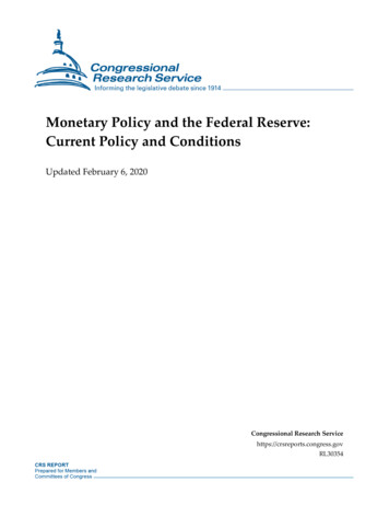
2.2.1. Post-crisis changes: liquidity regulationIn the standard model, a bank’s sole reason for demanding reserves is to satisfy reserverequirements. Banks’ liquidity risk management in the context of post-crisis regulations resultsin a new and independent source for demand for reserves by banks. For example, the liquiditycoverage ratio (LCR) requires banks to hold sufficient HQLA to meet net cash outflows over athirty-day stress period. HQLA include government securities and central bank reserves, as wellas some other safe and liquid assets. The LCR regulation implies that, compared to the pre-crisisperiod, banks’ demands for the sum of government securities and reserves increase. However, aswe discuss below, banks have a choice about how to allocate their HQLA between governmentsecurities and reserves; the LCR does not contain specific requirements about reserves per se. Inaddition, banks’ internal liquidity stress tests play an important role in the demand for reserves.Figure 3 illustrates the effect that liquidity risk management and regulation have on the demandfor reserves. Starting from the standard model’s demand curve, the liquidity regulation shifts outthe demand curve by the additional amount of reserves that banks choose to hold.In Figure 3, the outer demand curve labeled “maximum demand” represents the demand curvefor reserves if banks choose to satisfy their LCR requirements with reserves only. Banks couldchoose a different mix of reserves and other types of HQLA to satisfy the LCR requirements: Forexample, a bank may prefer to hold more reserves than government securities if the yields ongovernment securities are relatively low or if the bank thinks that it could be challenging toquickly convert government securities to cash in the face of outflows. And, of course, a numberof other considerations may be important.Since banks’ exact preferences are hard to determine from a central bank’s perspective, there isuncertainty in the amount of the increase in reserve demand due to liquidity regulations andbanks’ liquidity risk management. The inner demand curve represents the minimum demandcurve for reserves, where banks meet their LCR requirements mostly with other types of HQLAsuch as government and mortgage-backed securities rather than reserves. Importantly, thesecurves illustrate the perspective of the central bank or of a market observer, not that of anindividual bank. Any individual bank still has a single demand curve, located somewherebetween the inner and outer curves, but its location depends on a host of considerations that arecompletely known only to the bank itself.If the aggregate supply of reserves is given by 𝑆𝑆1 in Figure 3, then the interbank rate equals IORwith the minimum demand curve but exceeds IOR with the maximum demand curve. If,however, the aggregate supply of reserves is instead very large as given by 𝑆𝑆2 , then the interbankrate is equal to IOR for both the minimum and the maximum demand curves. Figure 3 reinforcesthe idea that the lower kink of the demand curve is an endogenous object and by extension so isthe idea of reserves being “scarce” or “abundant.” Uncertainty about the location of the kinkmatters more for market interest rates at intermediate levels of reserves. At sufficiently lowaggregate levels of reserves, the market rate will be rp regardless of which demand curve is ineffect; at sufficiently high aggregate levels of reserves, the market rate will be IOR regardless ofwhich demand curve is in effect. But at intermediate levels of reserves, the gap between the9

possible demand curves is larger and so is the uncertainty about the market interest rateassociated with a given aggregate supply of reserves.Figure 3: Effect of Demand Uncertainty.2.2.2. Post-crisis changes: balance sheet and trading costsOther post-crisis regulatory changes increased the regulatory costs of expanding a bank’s balancesheet or otherwise trading in money markets. One example is stricter rules on the leverage ratio.Another is that, in the United States, a bank’s Federal Deposit Insurance Corporation (FDIC) feeis currently based on the size of its balance sheet, while pre-crisis the fee was based on the sizeof the bank’s deposit liabilities.In the setup of the standard model, if a bank lends in the interbank market, its reserve holdingsfall but its balance sheet stays the same since the interbank loan replaces reserves as an asset onits balance sheet. If a bank borrows in the interbank market, its reserve holdings increase and its10

balance sheet expands. 11 On net, the aggregate balance sheet of the two banks expands. Thus,balance sheet costs act as an implicit tax on interbank trading and decrease trade volume in theinterbank market.Other post-crisis changes that are not technically balance sheet costs can also have the effect ofincreasing banks’ perceived cost of trading. For example, an enhanced focus on risk managementmay lead a bank to limit its positions with any one counterparty. Counterparty limits could thenprevent the bank from lending to some potential borrowers who value reserves more highly.Suppose for simplicity that the marginal implicit cost of interbank trading, c, is constant. Forexample, trading costs would take this form if a bank’s regulation fee increases by c when itsbalance sheet increases by a dollar. This sort of regulation drives a wedge between a (potential)borrowing bank’s demand curve and a (potential) lending bank’s demand curve for reserves,where the size of the wedge equals c (for details, see Kim, Martin and Nosal, forthcoming).Figure 4 illustrates demand cur

reserve supply can move money market rates by changing the scarcity value of reserves. At higher levels of reserves, where the demand curve has less or no slope, adjustments in administered interest rates become the main tool for moving money market rates. When a central bank faces shocks to reserve supply and demand, these differences in regimes