WIXLIB

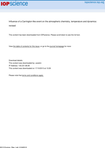
Environ. Res. Lett. 8 (2013) 045010M Calisto et alFigure 1. Height versus time evolution of ionization rates for the investigated solar proton event with the first impact at day 242 and thesecond impact at day 246. The upper panel shows the ionization from the 1956-type event, the lower panel from 1972, respectively. Thedata is given in ion pairs cm 3 s 1 .troposphere and lower stratosphere (Bazilevskaya et al 2008,Usoskin et al 2009). The CRAC:CRII model has been verifiedby comparison with available direct data sets and other models(e.g., Bazilevskaya et al 2008, Usoskin et al 2009). It does,however, underestimate the ionization above 30 km sinceit neglects UV irradiance (UVI) and precipitating particles(higher up in the polar atmosphere). On the other hand, theparameterization used in the papers by Rodger et al (2008)and Calisto et al (2012) stops at 20 km which makes it difficultto determine full ionization in the whole atmosphere (seefigure 1 for comparison of the IR).Moreover, the earlier models neglected variability of thebackground ionization due to the GCR, which may be veryimportant during strong geomagnetic disturbances (Usoskinet al 2011). Major geomagnetic disturbances are usuallyaccompanied by Forbush decreases (FD) of GCR, caused bythe same interplanetary transients (often a CME-driven shockwave). Although there is no clear general quantitative relationbetween the geomagnetic disturbance and the magnitude ofa FD (Kane 2010), strongest geomagnetic storms (Kp 8)are related to major FDs (magnitude 10%) (Belov et al2001). Since the period of late August–early September 1859was characterized by very strong geomagnetic disturbances(Humble 2006, Shea et al 2006) with two peaks: on DOYs 240(telegraph disruptions and extended aurora—Humble 2006)and DOY 244–245 with Dst possibly reaching an extremevalue of 1760 nT (Tsurutani et al 2003), we expect thatat least two FDs would occur during that period leading toa strong suppression of the GCR flux. Although we cannotreconstruct exact magnitude and time profile of the FDs,we make a reasonable conservative assumption. We assumethat both FDs were typical strong FDs with the magnitudeof 15% for a polar NM, which is consistent with, e.g., theFD of August 1972. Second, we assume that the recoverytime of GCR intensity was 4 days, which is typical formoderate-strong FDs (Usoskin et al 2008). We note that thisis a conservative assumption as such an extreme geomagneticstorm may be accompanied by a larger FD.The parameterization of the ionization rates cannotbe directly used in CCM SOCOL, which has no explicittreatment of ion chemistry and requires the conversion ofthe ionization rates into NOx and HOx production rates.The energetic protons in a solar proton event are able to ionize air molecules, X2 p X 2 p e , producingfast secondary electrons (X N, O, and the star symbolizeshigh kinetic energy). These electrons can then dissociate thenitrogen molecule, N2 e 2N(4 S; 2 D) e, where N(4 S)is the electronic ground state of the nitrogen atom and N(2 D)is its electronic first excited state. Almost all of the N(2 D)atoms react with O2 , producing nitric oxide, N(2 D) O2 3

Environ. Res. Lett. 8 (2013) 045010M Calisto et alNO O (whereas collisional quenching of N(2 D) plays onlya minor role). Conversely, the ground state can undergo a‘cannibalistic’ reaction with NO, N(4 S) NO N2 O,leading to the destruction of NOx . Therefore, within SOCOLN(2 D) is immediately converted into NO, while N(4 S) isa regular species in the CCM, which is subject to a fullkinetic treatment. Following Brasseur and Solomon (2005),when dissociation of molecular nitrogen yields one N(4 S)and one N(2 D) atom, the net odd nitrogen production isextremely small: almost every N(2 D) atom produces one NOmolecule, but almost every N(4 S) atom immediately destroysone at these altitudes. Net production is provided only by thevery small fraction of N(4 S) atoms which react with oxygen,N(4 S) O2 NO O, rather than with NO.Therefore, a quantification of the N(2 D):N(4 S) branchingratio is required. Following Porter et al (1976), 1.25 Nmolecules are produced per ion pair, of which 55% are N(2 D)and 45% are N(4 S) (see table V in Porter et al 1976). InSOCOL, the first excited state, N(2 D), is assumed to convertinstantaneously to NO. It is important to note that in the modelused here, the ground state atom, N(4 S), may undergo thecannibalistic reaction with the produced NO, i.e. N(4 S) NO N2 O, or may react, though much more slowly, withmolecular oxygen to generate NO. The production of HOx hasbeen taken into account using the calculations by Solomonet al (1981). They showed that below 60 km altitude about2 HOx molecules are produced, dropping towards 1.2 HOx at80 km. Egorova et al (2011) showed that the NOx and HOxparameterizations used in our study compare reasonably wellwith their model using complete ion chemistry.In order to simulate the SPE event, we have performedthe followed analysis. First we assumed that the event issimilar to the Carrington event in 1859 in the fluenceof 30 MeV (F30 1.9 1010 cm 2 ) as estimated byMcCracken et al (2001). The time profile of injection wastaken as proposed by (Shea et al 2006, figure 12 therein) withtwo injections, a smaller one peaked on DOY 240–241 anda major one peaked on DOY 245. Even though the existenceof the Carrington SPE is now doubted (Wolff et al 2012), westill consider it as the worst case scenario. Then we assumethat such a hypothetical event occurred in the year 2020.In order to model the atmospheric effect of such an eventwe consider two spectral shapes of the SPE energy spectra.A hard spectrum as for the event of February 1956, and asoft spectrum as for the event of August 1972 (see detail inUsoskin et al 2011). Then these spectra were scaled to matchthe SPE fluence proposed for the Carrington-like event. Wewill regard to these two cases as the hard spectrum (HS)and soft spectrum (SS) scenarios, respectively. These twoscenarios were then applied to the 3D CCM SOCOL v2.0. Wethen carried out three 9-month long runs—a control and twoperturbed runs—with ten ensemble members each, startingwith atmospheric conditions in August 2020 and ending inApril 2021. The ensemble members have been generated bysmall perturbations ( 0.1– 0.1%) of the CO2 mixing ratioduring the first month of the model run. We can comparethe Carrington event ionization rates to other SPEs, and asan example we have chosen the October 2003 SPE, which isone of the largest SPEs recorded and for which we have theionization rates readily available (they have been published,e.g., in Verronen et al 2005). We integrated the ionization ratesover the duration of the event, so that we can compare thetotal number of ion pairs produced at each altitude. We findthat at 35–60 km the total rates of the Carrington event are4–4.5 times higher than those of October 2003. This numberis similar to the scaling factor used by Thomas et al (2007),although they used a different SPE.3. ResultsThe ionization rates for the HS and the SS scenarios applied inthis study are shown in figure 1, suggesting that the major partof the energy is deposited in the stratosphere (20–40 km inaltitude). The characteristics of this solar proton event resultsin two distinct peaks, with the second peak stronger than thefirst one at the end of August. We can see that in the upperpanel, showing the IR for the HS case, the signal penetratesdown to the troposphere whereas the lower panel shows usthat the signal hardly reaches down to 10 km.Figures 3 and 4 as well as 6 and 7 show time seriesof zonal mean ensemble responses in NOx , HOx , ozone andtemperature. Figure 5 depicts the response of the HNO3 fluxin the SH averaged over the first month after the event.These results are calculated as a relative deviation of theexperimental run for the HS scenario and from the referencerun, i.e. the run without the influence of the energetic particles.The results obtained with the ionization rates for the SSscenario derived from Usoskin et al (2004) and Usoskin andKovaltsov (2006) will be discussed later in this chapter whencomparing them to the results with IR for the HS scenario.The results for NOx (see figure 3) show that theenhancement after this event lasts for weeks after theimpact happened, i.e. the changes in odd nitrogen in bothhemispheres are visible for about nine weeks. During thesolar proton event, a statistical significant increase, computedwith the Student T-test, of up to 2000% ( 80 ppbv) isvisible in the Northern Hemisphere (NH). In the SouthernHemisphere (SH), the maximum increase of up to 10 000%is shown in the upper troposphere/lower stratosphere (UT/LS)region, whereas an increase of more than 300% ( 70 ppbv)is depicted in an altitude range from 80 down to 60 km.The increase in NOx and the longevity of the changes arepretty similar when comparing this result with figure 2 inCalisto et al (2012), even though in this work, the most intenseincrease of NOx in the SH is depicted at the UT/LS region( 20 km). The reason for that can be explained with figure 2.There we see the peak of ionization in an altitude of about23 km.Figure 4 showing the changes in HOx depict an increaseof up to 600% in the NH and an increase of up to 4000%in the SH. This difference is caused by the fact the northernhemisphere has still a higher illumination compared to thesouthern hemisphere, i.e. the background level of HOx islarger (Rodger et al 2008). The results by Rodger et al (2008)are in good agreement when looking at the pattern of the HOx4

Environ. Res. Lett. 8 (2013) 045010M Calisto et alFigure 2. Red and rose lines: ionization rates (ion pairs producedper cm3 and second) as computed by the CRAC CRII model(Usoskin et al 2010). Blue line: ionization rate used in the papers byRodger et al (2008) and Calisto et al (2012).increase, i.e. the SH shows a more intense enhancement thenthe NH.This additional input of NOx and HOx , especially in thesouthern hemisphere, is able to change the HNO3 depositionfluxes as a response to the Carrington-like event, as we cansee in figure 5 which is averaged over the first month afterthe event. The statistically significant (at better than 95%level) response of up to 50% is simulated in the vicinity ofthe south pole. The response to this event is less pronouncedin the northern hemisphere (not shown). This hemisphericalasymmetry is related to the much higher intensity of HNO3sources in the NH in comparison with the relatively cleanhigh latitudes in the SH. The model includes dry and wetdepositions of O3 , CO, NO, NO2 , HNO3 , and H2 O2 . Thedry deposition flux or the removal rates by the absorption ofthe species at the surface is proportional to the predefineddry deposition velocities which are prescribed for differenttypes of surfaces following Hauglustaine et al (1994) and theconcentration of the species in the lowest model cell. Thedry deposition fluxes of several species from nitrogen group(NO, NO2 , HNO3 and N2 O5 ) are accumulated and stored asmonthly mean for all model cells. In addition, the removal ofthe soluble HNO3 by tropospheric precipitation is representedby a constant removal rate of 4 10 6 s 1 . The wet depositionfluxes are not stored.Losses in ozone of up to 60% and about 40% are visiblein the southern and the northern hemisphere, respectively(figure 6). These losses are correlated to the increase in NOxand HOx shown in figures 3 and 4 causing a depletion ofO3 from 80 down to about 30 km. Figure 7 depicting thechanges in temperature shows a decrease of about 1 K at about50 km in the northern hemisphere caused by the depletion ofozone which in turn leads to a decrease in solar heating inthe sunlit atmosphere. Contrariwise, the southern hemispherewhich shows stronger response in the other species, shows nostatistical significant cooling. The SPE induced cooling in thepolar region increases the pole to equator temperature gradientwith repercussion for the zonal winds.Figure 8 shows the changes in zonal winds averaged fromAugust to November for the NH and the SH at 30 hPa (upperpanel) and 50 hPa (lower panel). We see at both altitudes astatistical significant increase of up to 2 ms 1 in the northernhemisphere in the polar region. The acceleration of the zonalwind is explained by the fact, that we have a cooling inthe upper polar stratosphere due to the ozone depletion inFigure 3. Upper panel shows the changes in NOx zonal meanmixing ratio profile in the polar region (70–90 N). The lower panelshows the same for 70–90 S. Both panels show the results with theIR from 1956. Colors indicate areas with at least 95% statisticalsignificance. Upper panel contour levels: 20, 0, 20, 200, 700,1200, 2000, 10 000%. Contour levels lower panel: 20, 0, 20, 100,300, 800, 1000, 2000, 5000, 10 000%.Figure 4. Upper panel shows the changes in HOx zonal meanmixing ratio profile in the polar region (70–90 N) in per cent. Thelower panel shows the same for 70–90 S. Both panels show theresults with the IR from 1956. Colors indicate areas with at least95% statistical significance. Upper panel contour levels: 50, 20,0, 10, 50, 100, 150, 400, 600%. Contour levels for the lower panel: 50, 20, 0, 20, 80, 250, 800, 2000, 4000%.this region (see figures 6 and 7), which in turn leads to anacceleration of the zonal wind in agreement with the thermalwind balance (Limpasuvan et al 2005). The SH zonal windsseem not to be affected by SPE, we do not have similareffects as we have seen in the northern hemisphere. Thereason for that can be explained with figure 7, there we havenegligible changes in the temperature due to the solar protonevent. Therefore, no changes in the equator–pole temperaturegradient.5

Environ. Res. Lett. 8 (2013) 045010M Calisto et alFigure 7. Upper panel shows the changes in zonal meantemperature for the polar region (70–90 N) in Kelvin. The lowerpanel shows the same for 70–90 S. Both panels show the resultswith the IR from 1956. Colors indicate areas with at least 95%statistical significance. Contour levels: 6, 3, 1, 0, 1, 2, 3, 5,10 K.Figure 5. The response of the HNO3 deposition fluxes (%) in thesouthern hemisphere averaged over the first month after the eventfor the 1956 case. Over the stripped area obtained responses are notsignificant at a 95% confidence level.show the same for the IR for the SS case. This figure reveals,that for January, the ionization for the HS case has a statisticalsignificant warming of up to 7 K over Europe and Russiawhereas the ionization for the SS scenario shows neither astatistical significant increase nor a decrease over the abovementioned area. The southern hemisphere, however, showsfor both ionization scenarios a negligible decrease north ofAntarctica in January. The right side of the panel, showingFebruary, shows still a significant increase over Russia forthe IR for the HS whereas the ionization rate for the SSscenario has no statistical significant area over this part ofthe northern hemisphere. The southern hemisphere still showsjust a negligible decrease for the soft spectrum ionization rate.The general pattern for both ionization rates are in acomparable manner, i.e. they both show a warming overEuropa, Russia and the northern part of America in Januaryand February but the intensities and the significance arenot the same. Additionally, we see that the effects of theCarrington-like event result in an alternating cooling/warmingpattern resembling the typical response of the SAT caused bythe intensification of the polar vortex known as the positivephase of Arctic oscillation (Thompson and Wallace 1998),termed AO .Finally, we investigate the influence of such a major solarproton event on the total ozone (TOTOZ) for January andFebruary for both parameterization. The effects on TOTOZfor both hemispheres are displayed in figure 10. The upperpanel shows the total ozone, given in DU, for the HS caseionization for January and February whereas the lower panelshows the same for the SS scenario IR. We can see thatthe upper part of this figure depicts a statistical significantdecrease of more than 20 DU over Europe and Russia and asignificant increase of up to 30 DU over Canada. Other smalldecreases are visible but with a lower intensity. Interestingly,Figure 6. Upper panel shows the changes in ozone zonal meanmixing ratio profile in the polar region (70–90 N) in per cent. Thelower panel shows the same for 70–90 S. Both panels show theresults with the IR from 1956. Colors indicate areas with at least95% statistical significance. Contour levels: 80, 60, 40, 10,0, 5, 10, 50%.3.1. Comparison of the ionization rates for the hard and thesoft spectrum scenariosAs one can see in figures 1 and 2, the ionization rates for theHS and SS scenarios show differences not only in the intensityof ionization but also in how deep the particles penetratein the atmosphere. It is important to simulate events withdifferent spectra to analyze the difference between them. Theimportance of how deep the ionization penetrates is visiblein figure 9 where the surface air temperature (SAT) is shown.The upper panels represent the SAT for the ionization rates forthe HS scenario for January and February, the lower panels6

Environ. Res. Lett. 8 (2013) 045010M Calisto et alFigure 8. Upper row: polar stereographic projection of zonal wind changes at 30 hPa from August to November given in ms 1 . Lower row:zonal wind changes at 50 hPa from August to November given in ms 1 . Left column: NH. Right column: SH. Hatched areas show 95%statistical significance.Figure 9. Effect of solar proton event on SAT, [SAT]experimental-[SAT]reference, given in Kelvin for monthly mean. Upper panels: usingthe ionization rate from 1956 for January (left) and February (right). Lower panels: using the ionization rate from 1972 for January (left)and February (right). Hatched areas indicate changes with at least 95% statistical significance.the lower part of the figure, showing the IR for the SS case,shows just a small area of significant decrease over Europeand no significant increase over Canada, even though havinga larger area of increase. Both ionization show a small, i.e. upto 12 DU increase over Antarctica. When analyzing February,we can see that there is still a decrease of up to 20 DU7

Environ. Res. Lett. 8 (2013) 045010M Calisto et alFigure 10. Effect of solar proton event on TOTOZ, [TOTOZ]experimental-[TOTOZ]reference, given in DU for monthly mean. Upperpanels: using the ionization rate from 1956 for January (left) and February (right). Lower panels: using the ionization rate from 1972 forJanuary (left) and February (right). Hatched areas indicate changes with at least 95% statistical significance.4. Discussion and conclusionvisible over Europe and Russia but the area is not as big asin the January plot. The lower plot, showing the IR for theSS case for February shows small areas of decrease with amaximum of 8 DU. These ozone changes are not predictedto occur during the time when the event is happening; rather,the transport of the enhanced odd nitrogen to lower altitudesand therefore higher ozone amounts allows a more substantialtotal ozone impact. When the polar vortex breaks up, air fromlower la

2 Sodankylae Geophysical Observatory (Oulu unit) and Department of Physics, University of Oulu, FI-90014 Oulu, Finland 3 Physical-Meteorological Observatory/World Radiation Center, Davos, Switzerland 4 Institute for Atmospheric and Climate Science ETH, Zurich, Switzerland E-mail:Marco.Calisto@issibern.ch Received 25 June 2013