Transcription
Università degli Studi diPadovaFacoltà diIngegneriaDipartimento di Tecnica e Gestione dei SistemiIndustrialiCOMPUTER SIMULATIONANDARENA SOFTWARERelatore: Ch.mo Prof. Giorgio Romanin JacurLaureando: Iacopo MazziAnno Accademico2010/20111
TABLE OF CONTENTSSUMMARY . 5CHAPTER 1: INTRODUCTION TO SIMULATION . 61.1 INTRODUCTION. 61.2 COMPUTER SIMULATION . 71.2.1 PROS AND CONS OF COMPUTER SIMULATION . 71.2.2 DIFFERENT KINDS OF SIMULATION . 7CHAPTER 2: QUEUEING THEORY . 82.1 BASES OF QUEUEING MODELS . 82.2 LABELLING OF QUEUEING MODELS . 92.2.1 FORMAL MODEL OF M TYPE ARRIVALS . 92.2.2 FORMAL MODEL OF M TYPE SERVICE . 102.3 M/M/S QUEUES . 10CHAPTER 3: FUNDAMENTAL SIMULATION CONCEPTS . 113.1 PROBABILITY DISTRIBUTIONS . 113.1.1 DISCRETE DISTRIBUTION . 123.1.2 ERLANG DISTRIBUTION . 123.1.3 EXPONENTIAL DISTRIBUTION . 133.1.4 NORMAL DISTRIBUTION . 133.1.5 TRIANGULAR DISTRIBUTION . 143.1.6 UNIFORM DISTRIBUTION . 143.1.7 WEIBULL DISTRIBUTION . 153.2 PARTS OF A SIMULATION MODEL . 163.2.1 ENTITIES . 163.2.2 ATTRIBUTES . 163.2.3 VARIABLES . 162
3.2.4 RESOURCES . 173.2.5 QUEUES . 173.2.6 EVENTS . 173.2.7 SIMULATION CLOCK . 183.2.8 STATISTICAL ACCUMULATORS . 183.3 OVERVIEW OF A SIMULATION STUDY . 183.4 BUILDING A SIMPLE MODEL . 193.4.1 THE CREATE MODULE . 203.4.2 THE ENTITY DATA MODULE . 203.4.3 THE PROCESS FLOWCHART MODULE . 213.4.4 THE DISPOSE MODULE . 213.4.5 DYNAMIC PLOTS . 213.4.6 RESOURCE ANIMATION . 23CHAPTER 4: A BASIC MODEL . 254.1 AN ELECTRONIC ASSEMBLY AND TEST SYSTEM . 254.1.1 SYSTEM DESCRIPTION . 254.1.2 BUILDING THE MODEL . 264.1.3 RUNNING THE MODEL . 324.1.4 VIEWING THE RESULTS . 344.2 THE ENHANCED ELECTRONIC ASSEMBLY AND TEST SYSTEM . 364.2.1 SYSTEM DESCRIPTION . 364.2.2 SCHEDULES AND STATES . 364.2.3 RESOURCE FAILURES . 384.2.4 FREQUENCIES . 394.2.5 RESULTS . 40CHAPTER 5: A REALISTIC MODEL . 415.1 SYSTEM DESCRIPTION . 415.2 MODELING APPROACH . 433
5.3 BUILDING THE MODEL . 445.3.1 DATA MODULES . 445.3.2 LOGIC MODULES . 475.4 SYSTEM ANIMATION . 535.5 SYSTEM OVERVIEW . 55CONCLUSION . 57REFERENCES . 59ACKNOWLEDGEMENTS . 604
SUMMARYIn modern world simulation has become a fundamental tool in analyzing real lifesituations. Creating a model can sometimes be the only way to study a project andmost of times it is the most fruitful method.Through simulation it is possible to manage bottlenecks, improve order-managementsystems and to estimate warehouse capacity testing different plausible scenarios toimprove the process before running the real system.The aim of this work is first explain basic concepts of simulation, and in particularcomputer simulation, and then apply them to concrete situations, from the simplest tothe more realistic ones.The expected result is to give the reader a basic knowledge of how simulation can behelpful in different occasions and to provide the means to create basic andintermediate realistic models.5
CHAPTER 1: Introduction to simulation1.1.IntroductionSimulation attempts to model real-life or hypothetical situations to study how thesystem works, usually with appropriate softwares.Computer simulation deals with models of systems. A system can be defined as aprocess, either actual or planned.Examples of different systems can be: A distribution network of plants, warehouses and transportation links; A supermarket with inventory control, checkout, and customer service; A manufacturing plant with machines, people, transport devices, conveyor beltsand storage space.Sometimes it might be possible to experiment with the actual physical system, likeexperimenting with different traffic lights sequences, but sometimes it is too difficult,costly or impossible to do physical studies on the system itself like in the case of anexisting factory (it might be extremely costly to change to an experimental layout).Two of the most important kinds of models that can be highlighted are: physical modelsand logical (or mathematical) models: Physical models can be both tabletop models that are miniature versions of thefacility and a full-scale version simulating the facility itself. Logical (or mathematical) models are usually represented in a computer programthat is exercised to address questions about the model’s behavior.If the model is simple enough it is possible to use traditional mathematical tools likequeueing theory, differential-equation methods or linear programming but mostsystems subject of study are so complicated and may not be possible to find exactmathematical solutions, which is where simulation comes in.In this discussion will be analyzed only logical models using a simulation software,Arena by Rockwell Automation.6
1.2.Computer simulation1.2.1.Pros and cons of computer simulationComputer simulation refers to methods for studying a wide variety of modelsreproducing a wide variety of real-world systems by numerical evaluation; in the lastthree decades simulation has been considered as the most powerful and popularoperations research tool. The reason for this is that the model can be allowed tobecome extremely complex, so it can represent faithfully the system while othermethods may require stronger simplifying assumptions about the system to enableanalysis, which might bring the validity of the model into question.On the other hand simulation is not always as easy as it seems: many real systems areaffected by random inputs, and consequently many simulation models involvestochastic input components causing their output to be random too.1.2.2.Different kinds of simulationThere are many different ways to classify simulation models, but a useful way is alongthese three dimensions: Dynamic or Static: Time plays a natural role in static models but does not in staticones. Most operational models are dynamics and Arena was designed to best fitwith this kind of models. Discrete or Continuous: In a discrete model changes occur only at specifiedpoints in time while in a continuous model the state of the system changescontinuously over time. A discrete model can be a manufacturing system whereparts arrive and leave following a specific timetable; a water reservoir with waterflowing in and out is a perfect example of a continuous model. In the same modelcan be present elements of both discrete and continuous change: these modelsare called mixed continuous-discrete models. Deterministic or Stochastic: Models with no random inputs are calleddeterministic models while stochastic models operate with at least some randominputs. Due to the randomness of the inputs, even the outputs of a stochasticmodel are uncertain and the analyst has to consider this carefully in designingand interpreting the results of this kind of projects.7
CHAPTER 2: Queueing theory2.1.Bases of queueing modelsQueues (or waiting lines) are necessary when customers wait for a service as theservice capacity is not sufficient to supply the service at once.In a queueing model: Customers are generated by an input source. Customers arrive according to an arrival rule. Customers enter the system by joining a queue. A customer is chosen according to a queue discipline. The chosen customer obtains the required service. The service follows a service rule. The customer who obtained the service exits the system.SourceArrival ruleQueueService ruleServiceExitThe input source may have either infinite or finite population; if the population is infiniteit is not altered by additional customers entering the system.Customer arrival is ruled by the interarrival time distribution.Queues may be either infinite or finite (in this case we cannot exceed a maximumcapacity).Queue discipline may be FIFO (First In First Out), LIFO (Last In Last Out), SIRO(Service In Random Order), sorted (according to a priority), PS (Processor Shared) orAS (Ample Server).It is possible to have one or multiple servers; if multiple we have parallel servicechannels.8
2.2.Labelling of queueing modelsQueueing models can be represented using Kendall’s notation:A/B/S/K/N/D.“A” is the interarrival time distribution (or arrival rule), “B” is the service time distribution,“S” is the number of servers (parallel channels), “K” is the maximum system capacity orthe maximum number of customers in the system, “N” is the source population and “D”is the service discipline assumed (FIFO, LIFO, SIRO, PRIOR, PS or AS).Some standard notation for interarrival time and service time distributions are: M for amemoryless or Markovian (exponential) time, G for general (arbitrary) time, D fordegenerate distribution and Ek for an Erlang distribution with k phases.By default the service discipline is considered as First In First Out (FIFO), while bothsystem capacity and source population are assumed as infinite so, using Kendall’snotation, we can have for example M / M / 1 or M / G / 1 or M / M / S.2.2.1.Formal model of M type arrivalsGiven 0 as current instant, t as any instant 0 and τ as the instant of next arrival, theprocess may be described in two equivalent ways:Where λ is a positive real number and o(Δt) is an infinitesimal of upper order withrespect to Δt.Obviously the interarrival time is exponentially distributed, λ is the arrival rate, or themean number of arrivals in time unit and 1/λ is the mean interarrival time.The value of λ may be a constant (infinite source population and homogeneous systemwith infinite capacity), dependent on the number of customers in the system (finitesource population or finite capacity of the system)
In this discussion will be analyzed only logical models using a simulation software, Arena . Arena software contains various built-in functions for generating random variates from the commonly used probability distributions. Each distribution has in Arena one or more parameter values associated with it and is required to specify these parameter values. 1 1 1 .