Transcription
Chapter 2The Relation Between Classical and QuantumStatisticsThe definition of thermal average values in the canonical ensemble as a sum overall states with a Boltzmann factor as the weight, given in Eq. (1.68), is rigorous.It is also useful insofar as we can actually calculate the levels and their propertiesquantum mechanically. This is possible for a number of Hamiltonians but certainlynot for all interesting ones. Happily there will often be an alternative in the formof a classical treatment. A classical description of a system requires that quantumnumbers are big compared to unity and is useful because one needs not know alldetails of the system to apply it.There are two approaches to explain the classical-quantum statistics connection.One may either start from the truth as we have learned it at school, that quantumstatistics is fundamental and classical statistics can be derived in the classical limit,the ‘bottom-up’ approach. Alternatively, one can use a more historical approachand start with classical dynamics and postulate certain rules which will turn out togive the right result, the ‘top-down’ approach. We will do both. One advantage ofthe ‘bottom-up’ approach is that it provide some training in the ensembles that wereintroduced in Chap. 1. The main but not exclusive virtue of the ‘top-down’ approachis conceptual; you will be wiser after having understood the procedure.As an essential step towards application of the classical equations of motion anddetermining the range of validity of the results, we need to establish the rule whichrelates the classical and the quantum mechanical counting of states. We also needto consider the special quantum mechanical effects of the indistinguishability ofparticles. We will start with the latter.Quantum statistical mechanics is influenced in an essential manner by the symmetry of the wave function upon permutation of the particles. It is well known fromquantum mechanics that fermions of the same type (half-integer spin particles, electrons being the prime example) are described by a wave function that must be antisymmetric on exchange of any two fermions. This has the consequence that twoidentical fermions cannot be in the same single particle quantum state. This ruleis absolutely essential for the description of the types of matter where bound stateelectrons are involved, be it in atoms, molecules and solids, and whether these solidsare metals or insulators. Basically the Pauli exclusion principle, as the rule is called,K. Hansen, Statistical Physics of Nanoparticles in the Gas Phase,Springer Series on Atomic, Optical, and Plasma Physics 73,DOI 10.1007/978-94-007-5839-1 2, Springer Science Business Media Dordrecht 201327
282The Relation Between Classical and Quantum Statisticsprohibits most of the states one would otherwise include in a counting of states. Foridentical bosons (integer spin particles) an analogous rule applies, except that thewave function must be symmetric. This means that bosons are social particles andwill tend to cluster together. The consequences of this is probably best known forthe Bose-Einstein condensates which you can read about in press releases from theNobel committee. But even everyday objects like lasers(!) work precisely becauseof this social tendency (photons are bosons).Quantum mechanically, identical particles are indistinguishable. Even in the classical limit, the partition functions therefore needs to be divided by the number ofpermutations of the number of particles in the system. For N identical particles thefactor is N ! Hence the canonical partition function of N indistinguishable particleswith the single particle partition function z iszN,(2.1)N!which we have already used in the Introduction. The factor of N ! appears only ifthe particles really are indistinguishable, which means that it will be applicable fora gas but not for atoms in a solid, where the atoms can be identified by their positionin the lattice. Molecules in a gas will move around freely apart from infrequentcollisions with other molecules and possibly the walls of a container, and after sometime it becomes impossible to determine the position of a specific molecule, evenclassically.As indicated, indistinguishability may be a time dependent question. We canspeculate on the time scales. If we perform a Gedanken experiment where we measure the positions of gas molecules at some specific time such that we can tell themapart at the time of measurement, even if they are otherwise indistinguishable, theentropy will be less than before the measurement. For the sake of the argument weassume that the measurement is made such that the wave functions of individualmolecules collapse to Gaussian wave packets, and for simplicity consider the subsequent development in one dimension only. The wave packets spread out as 2 p 22t .( x) x(0) (2.2)mZN For a Gaussian wave packet, p /2 x(0) and we can therefore express x interms of x(0) and time as 2 2 t .( x)2 x(0) (2.3)2m x(0)We can find the time it takes for two identical molecules to have a quantum mechanical overlap and become indistinguishable. This time depends on x(0). Thelongest value of this time for two particles a distance d apart corresponds to x(0) d/2 2 and is equal to t md 2 /8 m/ ρ 2/3 , where m is the mass of theparticle and ρ the gas density. For an ideal gas at Standard Pressure and Temperatureof P 1 bar 1.013 105 N/m2 , T 293 K, the time is t (m/1 u) 2 · 10 10 s.This is a short time but it is not zero.
2 The Relation Between Classical and Quantum Statistics29The example is a little artificial because the width of the wave packet correspondsto a very low kinetic energy. A more realistic estimate is obtained by using the2 1/22T /m. Under the sameaverage root-mean-square thermal speed p /m 1/3 2 · 10 12 s for a 1 uconditions as before, this gives t d m/T m/T ρparticle (the width of the wave packet can be ignored in this calculation, making iteffectively a classical calculation).In practise, this time dependence causes few problems for gases. For liquids, itmay be different because the motion of atoms is constrained, but not completelyhindered as in a solid at low temperature. The calculation of the thermal propertiesincluding the proper distinguishability factor may then be non-trivial and depend onthe specific molecular properties of the liquid state. We will leave this subject forfuture studies.A consequence of quantum statistics is that the counting of states is often muchmore complicated for a system with a fixed number of particles than for a system with a fixed chemical potential. In a grand canonical ensemble, with its fixedchemical potential and fluctuating particle number, the partition function is calculated with a summation over all particle numbers, with the chemical potential asthe constant price you pay for the addition of a single particle. In the canonical andmicrocanonical ensembles you need to restrict the summation to states that have precisely the right number of particles. This restriction of the summation is generallya non-trivial task. This means that the description of fermionic and bosonic systems usually is very cumbersome in the canonical ensemble and is best done withthe grand canonical ensemble. There are exceptions. Bosons such as photons andphonons are cases for which the canonical partition functions can often be calculated analytically. The feasibility of summing over states with the correct quantumstatistics is the one important property which makes the grand canonical ensembleuseful and in practice the ensemble of choice, even in cases where particle numbersare conserved. The practical, computational advantages of the ensemble can simplyoutweight this inconsistency.The cases where the grand canonical ensemble is particularly useful are thosewhere the system can be described in the independent particle approximation, i.e.where one can write the energies of the system as sums of single particle state energies, and when the system is a strongly degenerate fermionic or a bosonic system.Strongly degenerate means for fermions that the lowest energy single particle statesare occupied with a probability which is close to unity, and for bosons that a significant fraction of the particles are in the lowest energy state. For fermions, the energyof the highest occupied level at zero temperature is called the Fermi energy andis on the order of usual molecular electronic energies, i.e. several eV. For bosons,the highest occupied level at zero temperature is simply the ground single particlestate, which we can assign zero energy. For low enough temperatures we thereforehaveμ Ef(fermions)μ 0 (bosons).(2.4)(2.5)
302The Relation Between Classical and Quantum Statistics2.1 Fermi and Bose Statistics of Independent ParticlesFermionic and bosonic systems of independent particle states are prototype ‘bottomup’ situations and are the natural choices to illustrate a concrete application of thegrand canonical ensemble and the transition from quantum to classical statistics.Irrespective of whether a system is strongly degenerate or not, i.e. whether ornot the occupation number is small compared to unity or not, in the single particlepicture the total energy is given by E nj εj ,(2.6)jand the number of particles byN (2.7)nj ,jwhere nj is the occupation number of state j , i.e. the (integer) number of particlesin that single particle state. The canonical partition function is therefore Zcan (N, V , T ) δN, nj e β j nj εj ,(2.8)(n1 ,n2 ,.)where the sum runs over all combinations of the nj ’s consistent with the permutationsymmetry of the particles. The permutation symmetry requires thatni 0, 1(fermions)ni 0, 1, . . . , N 1, N(2.9)(bosons)The Kronecker delta δn,m , which is one if n m and zero otherwise, picks out theconfigurations with the right total number of particles in Eq. (2.8).The grand canonical partition function, Eq. (1.73), can therefore be written asZgcan δN, nj e β jnj εjeβμN .(2.10)N 0 (n1 ,n2 ,.)Summation over all values of N cancels the Kronecker delta because δn,m 1,(2.11)mand we can then sum unrestricted over all sets of occupation numbers, apart fromthe permutational symmetry constraint in Eq. (2.9): Zgcan e β j nj εj β j nj μ .(2.12)(n1 ,n2 ,.)The exponential can be factorized into contributions from each level, and one endswith a product of grand canonical partition functions for individual levels: e βnj εj βnj μ .(2.13)Zgcan jnj
2.1 Fermi and Bose Statistics of Independent Particles31This is valid for both fermions and bosons. The difference between the two showsup when one calculates the sums, taking the permitted particle numbers into account, Zgcan 1 e β(εj μ) (fermions, independent particles),(2.14)jandZgcan 1 e β(εj μ) 1(bosons, independent particles).(2.15)jOne may want to think of these two partition functions in a different way. They areformally identical to those of independent excitations with the spectraei,n n(εi μ),n 0, 1 (fermions),n 0, 1, 2, . . . , (bosons),(2.16)and the average occupation number is the thermal average of the excitation energyin units of εi μ.From the partition functions one finds the populations of the individual quantumstates to bee β(εj μ)(2.17)1 e β(εj μ)( for fermions, for bosons). These populations are illustrated in Fig. 2.1 forboth types of systems, both with 100 particles and with single particle states that areequidistant in energy, εj j , where j is a non-negative integer. Also shown arethe chemical potentials corresponding to 100 particles on the average, for the rangeof temperatures T 5 to 50.The stage is now set to find the classical limit of the thermal properties of thequantum gases. This limit is defined as the situation where the occupation numberof each state is much less than unity;pj e β(εj μ) 1.1 e β(εj μ)We can ignore the exponential in the denominator to get N e β(εj μ) eβμe βεj .pj j(2.18)(2.19)jThe sum is nothing but the canonical partition function for a single particle (identicalexpressions for a fermion and a boson), zc,1 , and we find that the chemical potentialisμ T ln(zc,1 /N ).(2.20)This chemical potential can be compared with the one calculated for a classical gasof indistinguishable molecules, Eq. (1.79), in Chap. 1. Apart from the replacementof a fixed number N of atoms with an average number, N , the two expressions areidentical. Because the chemical potential is the derivative of the canonical partitionfunction, this also mean that the classical limit of the (canonical) partition functions
322The Relation Between Classical and Quantum StatisticsFig. 2.1 The population insingle particle states forN 100 bosons (top frame)and fermions (bottom frame)in the grand canonicalensemble at temperatures 5 to50, for equidistant singleparticle spectra. The chemicalpotentials vs. temperature areshown in the insets. Allenergies and temperatures arein units of the spacing in thesingle particle spectrum, for non-interacting bosons and fermions have the same form as the classical limitwritten down in Chap. 1, Eq. (1.77). It is noteworthy that the indistinguishabilityfactor N ! appeared automatically here, without any need to introduce it by hand.Historical remark: The factor was postulated by Gibbs before quantum mechanicswas even an idea, in order to get the correct additivity of the entropy of a classicalgas.2.2 Classical Phase SpaceSo let’s turn to the second point of this chapter, the ‘top-down’ approach. In a quantum description of matter you have well-defined energy levels which can be numbered and counted. In classical mechanics this is not the case. An instructive example is (again) the harmonic oscillator. Quantum mechanically it has one more stateeach time the energy is increased by ω. Suppose you had not solved the quantummechanical problem and still had to decide the number of states of the system at acertain energy. What would you do?The solution is found when we take a closer look at the classical counterpartof the Hilbert space used in quantum mechanics. It is called phase space and is,
2.2 Classical Phase Space33like the Hilbert space, a multi dimensional space. Unlike Hilbert space it is notspanned by square integrable functions, but the coordinates and momenta of all theparticles in the system. These coordinates and momenta need not be the usual linearquantities you learn about in the first course on mechanics, but can be generalizedcoordinates and their conjugate momenta, for example an angle and its associatedangular momentum.A system of N particles will span a space with 6N dimensions, or more generally2dN dimensions if the physical space is d-dimensional. A state of the system isdefined as the point in this 6N dimensional space that specifies all the momentaand coordinates. The classical microcanonical partition function is the area of thesurface with the prescribed energy, embedded into this space. It does not sound as ifit is easy to calculate, and often it isn’t. The canonical partition function is easier. Itis calculated as the integral over the whole space with the Boltzmann factor as theweight function:Z exp βE(x1 , x2 , . . . , x3N , p1 , p2 , . . . , p3N ) dx1 dp1 dx2 dp2 · · · dx3N dp3N .(2.21)As an application of the classical distribution we will calculate a few results foran ideal gas. In an ideal gas the molecules do not interact with each other or anythingelse and the Hamiltonian is therefore a sum of the kinetic energies of all molecules,which for simplicity will be assumed to have the same mass m: p2iH .(2.22)2miThe Boltzmann factor therefore factorizes, and for every molecule the momentumdistribution isP (px , py , pz )dpx dpy dpz e βpx2 py2 pz22m(2.23)dpx dpy dpz . px2 The distribution is spherically symmetric in momentum space. With22py pz and integrating out the angular dependence, which just gives a multiplicative constant of 4π , we havep2p2P (p)dp p 2 e β 2m dp v 2 e βmv2 /2dv.(2.24)This is the Maxwell-Boltzmann distribution of momenta or speeds of gas moleculesin an ideal gas in three dimensions.The absence of intermolecular interactions is an unnecessary restriction. Anyrealistic Hamiltonian will contain terms that represent the interaction of the gasmolecules with each other or it may even describe a condensed phase where interactions are plentiful. As long as the interaction terms only depend on the positions andnot on the momenta/velocities of the molecules, the coordinates can be integratedout independently of the momenta,1 and consequently the velocity distribution isalso given by Eq. (2.24) for these situations.1 Inprinciple. In practise it is not that easy. This is another Gedanken calculation.
342The Relation Between Classical and Quantum StatisticsThe classical partition function in Eq. (2.21) still leaves out the value of the constant of proportionality. A suggestion of what that constant can be is found in thedimensions of Z. If we want to have any correspondence between the classical andthe quantum cases, we must at least demand that the dimensions of the two quantities are identical. The quantum partition function is dimensionless as it is a sum overexponentials. But the integral in Z in Eq. (2.21) has dimension of coordinate timesmomentum, all to the power 3N . If you calculate the dimensions of the product of acoordinate and its conjugate momentum you get the dimension of Planck’s constant.This is no accident. The normalization constant is 1/ h3N . In other words: one stateof a system with M sets of conjugate coordinates and momenta has a volume of hMin phase space. We can define a semiclassical canonical partition function asZsemiclass 1Zclass .h3N(2.25)It should be clear that this prescription only works for systems that actually have aclassical description. This rules out the application of Eq. (2.25) to spins and similardegrees of freedom.For many purposes the distinction between the semiclassical expression and thetruly classical partition functions is no problem because any multiplicative constantdrops out when calculating observables with logarithmic derivatives or comparingvolumes in phase space (of similar dimensionality). For calculation of entropies, itdoes count, however.Equation (2.25) can be derived with a calculation where the partition function isexpanded in powers of . The calculation will not be reproduced here. Instead, wewill show with several examples, at the end of this chapter, that the result holds andthen hope that the perfect agreement with our Ansatz applied together with exactcalculations will convince you that all other (classically meaningful) cases can betreated this way. Before that, we will calculate some general results for the classicallimit.2.3 A Few Elementary and Useful Results from ClassicalStatistical MechanicsThe classical partition function allows a simple estimate of the high energy/temperature limit of the thermal properties of the systems for which the classicallimit makes sense (a spin in a magnetic field wouldn’t work, for example). A coordinate, qi say, may appear in quadratic form uncoupled from other coordinates andmomenta in the Hamiltonian, H : (2.26)H αqi2 H q , p ,where p is the set of all momenta and q is the set of all coordinates except qi . Thecontribution to the canonical partition function from qi factorizes:
2.3 A Few Elementary and Useful Results from Classical Statistical MechanicsZ 1h3Ne βH dqj dpj j1 βαq 2i dqeih1h3N 11e β(αqi H ) dqi2h3Ne βH 35dqj dpjj dqj dpj ,(2.27)jwhere the primed product of differentials is the one where dqi is left out. The lastintegral is denoted Z and thenZ Z1he βαqi dqi .2(2.28)If qi can take all values, the integration over qi can be expressed in closed form;Z 1hπZ.βα(2.29)It should be clear that this holds for all degrees of freedom that separate the way qidid, coordinates and momenta alike. Consequently, the contributions to the partitionfunction from all those degrees of freedom will be proportional to 1/β T ,taken to a power which is this number of degrees of freedom. It is equally clear thatthe factorization does not depend on whether or not the Hamiltonian is quadratic inthe degree of freedom or has some other functional form, although the value of thespecific integral will.The average thermal energy of the system in the canonical ensemble isπd ln( h2 βα ) d ln(Z ) T d ln(Z) E , E dβdβdβ2(2.30)with the above meaning of the primed quantity. Hence the contribution to the thermal energy is T /2 from each degree of freedom that enters into the energy quadratically. With this result, the properties of the Maxwell-Boltzmann distribution canpractically be read off the Hamiltonian without any further work. The partition function for an ideal gas of N particles isZ β 3N/2 T 3N/2 ,(2.31)and the average kinetic energy E ln(Z) 3N T. β2(2.32)The 3 appears because of the number of independent momenta in space. The heatcapacity from these types of degrees of freedom is also easy to find. For one d.o.f.it is simply C 1/2 ( kB /2), and like the energy it is additive. Note that the valueof α does not appear in either of these quantities.These rules, known as equipartition, can be very useful because they quicklygive a value for the classical thermal energy and heat capacity. One use is to judge,from experimental data, whether certain d.o.f.’s are classical or not. Historically,equipartition was a problem for statistical mechanics because the heat capacity of
362The Relation Between Classical and Quantum Statisticselectrons in metals was observed not to obey this simple law. Not knowing the Pauliprinciple it was very difficult to explain the anomalously low heat capacity of thesecomponents of matter.Another simple observation can be very useful. If the level density can be writtenas a power of the excitation energy, the partition function is easily calculated to be: Z E s 1 e βE dE β s T s .(2.33)0The converse also holds; a partition function of the latter form will only arise froma powerlaw level density with the powers of the two related as s and s 1.2.4 Quantum Corrections to Interatomic PotentialsAbove we discussed how to convert the classical canonical partition function to thesemiclassical by division with a factor 2π to an appropriate power, and to accountfor the indistinguishability with the factor 1/N! In this section we will go a stepcloser to the quantum limit and calculate quantum corrections to the equations ofmotion for two particles interacting with a two-body potential.The classical motion of a particle represents it as a point moving on a trajectory.The correction we will calculate here amounts to treating it as a propagating wavepacket. The simplest of these are Gaussian. In x-space;φ eα(x x 0 )2 /2.(2.34)The probability distribution φ 2 for this wave function has the width 2 1. x 2αFor the momentum the width is equal to the thermal width: 2 p 2mEk 3mT .(2.35)(2.36)This relation expresses that the particle is not in a pure momentum or kinetic energy eigenstate, but rather in a superposition of kinetic energy eigenstates that hasa width determined by the temperature. Next we use the Heisenberg indeterminacyrelations, better known under the slightly more convenient names Heisenberg uncertainty relations, or uncertainty principle, to relate the width of the wave packet tothe temperature; p x .(2.37)2(The equality holds for a Gaussian wave packet.) This gives the shape parameter, α,of the wave packet in terms of the temperature:α 6mT. 2(2.38)
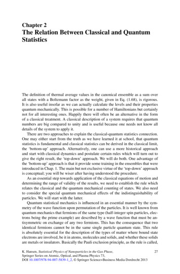
2.4 Quantum Corrections to Interatomic Potentials37Fig. 2.2 Two situations where the wave packet dynamics can (left) and cannot (right) be used.The potentials are quadratic and the wave packets are Gaussians. The energies corresponding tothe widths of the wave packets are given as dotted linesBecause we are dealing with two-body interatomic potentials, we will replace themass m with the reduced mass of the two identical mass particles, μ (m 1 m 1 ) 1 m/2, in the following.The next step is to place the wave packet on a potential energy surface, becausethis is what we are interested in. This introduces other length scales in the problem that may not be compatible with the one determined by T . Specifically, if thetemperature is low, the wave packet in Eq. (2.34) will be very broad and reachinto regions of very high energy. When the presumed wave packet spreads into regions with potential energies that are much higher than p 2 /2μ, it is a sign that theAnsatz Gaussian wave function is a poor description of the physical situation. Fora quantitative calculation of where this limitation sets in we use the example of aone-dimensional harmonic oscillator. We have the criterion: 1 2 2 1 2 2 p 2μω x μω.(2.39) 222 p2μThis requirement means that the potential energy associated with the width of thewave packet is less than the kinetic energy of the same. Using that the kinetic energy is half the total energy for a harmonic oscillator, p 2 /2μ E/2, we get thecondition1(2.40)E ω,2which looks like a reasonable condition. It tells us that we are dealing with a hightemperature approximation of the quantum contribution to the equations of motion.The condition is illustrated in Fig. 2.2.After having established the limit of the approximation, we proceed with thecalculation of the average potential. It is the average over the wave packet: Vqc (r) V r R φ 2 dR,(2.41)
382The Relation Between Classical and Quantum Statisticswhere V is the classical potential. The integrand is a function of the distance between the two atoms, although the integration is over a three dimensional space. Weperform the integral with an expansion to second order in the distance. First R isexpressed in polar coordinates with the z-axis along the line connecting the atoms, 1/2R2R2 R cos θ cos2 θ, r R R 2 sin2 θ (r R cos θ )2 r 2rr(2.42)where r r and similar for R, and terms to second order in R have been retained.We therefore have the expansion of the potential along the interatomic axis, retainingterms to the same order; 2 R2R12V V (r) V (r) R cos θ cos θ V R 2 cos2 θ · · · . (2.43)2rr2This gives the effective (quadratic Feynman-Hibbs) potential 6μ 26μ 3/22 β 2 RVQF H (r) edφdθsinθdRRπβ 2 2 R2R1 R cos θ cos2 θ V R 2 cos2 θ . V (r) V (r)2rr2(2.44)The integrals are standard. We get 22VV .(2.45)24μTrThis is the effective two-body potential in the high energy limit for the classicalpotential V .VQF H (r) V (r) 2.5 Example 1: The Harmonic OscillatorWe will now give a few examples of the classical limit of thermal properties of single particle systems with known or traceable quantum mechanical properties. Firstthe harmonic oscillator. The canonical partition function for a quantum harmonicoscillator is one of the simplest to calculate. It isZqm e βn ω n 0At high temperatures, Tthe classical limit:Zqm 1.1 e β ω(2.46) ω, the average quantum number is big and one reaches1(β ω)221 (1 β ω · · ·) ωT1T1 . ω2T ω 2 1β ω(1 β ω2 · · ·)(2.47)
2.5 Example 1: The Harmonic Oscillator39The next-to-leading term of 1/2 is the same 1/2 which appeared in the improvedformula for the level density, Eq. (1.28).Let’s now calculate the classical partition function. The energy isp21 mω2 x 2 .2m 2Inserting this into Eq. (2.21) we have:E Zclass dx p2(2.48)1dp e β( 2m 2 mω2x2).(2.49)The exponential factorizes into two parts which depend on x and p alone. We therefore end up with two Gaussian integrals that can be done:2 1e β 2 mω p2e β 2m dp 2 1 x 22m p 22πTedxedp . (2.50) βm ω β ωZclass 2x2dxIf you compare this with the leading order in Zqm from Eq. (2.47) you see thatthe missing constant of proportionality is h:1Zqm Zclass .(2.51)hAt least our rule in Eq. (2.25) holds for the harmonic oscillator.We can use semiclassical quantum physics to understand the origin of this rule.Semiclassical quantization uses classical equations of motion but accept only solutions where the trajectories obey a certain quantization condition. According to thistheory, the energy of a harmonic oscillator is quantized asp21(2.52) mω2 x 2 n ω,2m 2where n is a non-negative integer. This equation defines a curve in phase spacewhich is an ellipse and on which the semiclassical harmonic oscillator moves. Thelength of the two axis are determined by solving Eq. (2.52) with p 0 and x 0for the biggest values of the coordinate x and the momentum p with the result 2 1/2xmax n ω,pmax (n ω2m)1/2 .(2.53)mω2We can find the volume in phase space, Vn , of the lowest n 1 states that have thequantum numbers from 0 to n, as the area of the ellipse:E Vn πxmax pmax π2n ω nh.(2.54)The volume in phase space of state n is then nh (n 1)h h. It is illustrated inFig. 2.3.2 If we are average physicists, that is. As Predrag Cvitanovic remarked, a Gaussian integral is theonly integral an average physicist can do (Classics Illustrated: Field Theory, NORDITA Lecturenotes, 1983).
402The Relation Between Classical and Quantum StatisticsFig. 2.3 The phase space ofa single harmonic oscillator.The states permittedaccording to semiclassicalquantization are drawn aslines. The area between eachline is constant and equal to hAs the alert reader will have noticed, the ground state is not represented correctly this way. This is a general problem, both with semiclassical quantization andwith the classical partition function. At energies comparable to or below the lowestexcitation energy, the classical partition function should not be used.2.6 Example 2: A Free ParticleThe free particle is particularly important because it is frequently encountered.There are no discrete quantum numbers associated with the translational motion,and we need a trick to calculate the lev
Chapter 2 The Relation Between Classical and Quantum Statistics The definition of thermal average values in the canonical ensemble as a sum over all states with a Boltzmann factor as the weight, given in Eq. (1.68), is rigorous. It is also useful insofar as we can actually calculate the levels and their properties quantum mechanically.