WIXLIB

Proceedings of the Thirtieth International Joint Conference on Artificial Intelligence (IJCAI-21)Collaborativegraph ologygraph𝐞𝐯𝐯𝛼Note Temporal visitlearning𝐫disease𝐨𝛼word𝛼 𝐫 𝐲𝑡𝐯𝛼patient𝛼𝐨Figure 2: An overview of the proposed model. The graph learningfirst learns disease hidden features with two collaborative graphs: anobservation graph and an ontology graph, based on the hierarchicalembedding from medical domain knowledge. Then an RNN is designed to learn temporal information of visit sequences. RectifiedAttention mechanism encodes clinical notes with the guide of TFIDF and uses the visit representation as an attention context vectorto integrate structured visit records and unstructured clinical notes.child nodes for each non-leaf node to pad them into virtualleaf nodes. We assume there are nk nodes at each level k(smaller k means higher level in the hierarchical structure).We create an embedding tensor {Ek }k [1,2,.,K] for nodesin the tree. Ek Rnk dc is the embedding matrix for nodesin level k, and dc is the embedding size. For a medical codeci as a leaf node, we first identify its ancestors in each levelk [1, 2, . . . , K 1] in the tree and select correspondingembedding vectors from {Ek }. Then, the hierarchical embedding ei RKdc of ci is calculated by concatenating theembeddings in each level: ei Ei1 Ei2 , . . . , EiK ,where denotes the concatenation. We use E R C Kdcto represent medical codes after hierarchical embedding.Graph RepresentationIn visit records, specific diagnosis co-occurrences could reveal hidden similarities of patients and diseases. We exploresuch relationship by making the following hypotheses:1. Diagnostic similarity of patients. If two patients get diagnosed with the same diseases, they tend to have diagnostic similarities and get similar diagnoses in the future.2. Medical similarity of diseases. If two diseases belongto the same higher-level disease, they might have medicalsimilarities such as symptoms, causes, and complications.Based on these hypotheses, we construct a collaborativegraph G {GU C , GCC } for patients and medical codes. GU Cis the patient-disease observation graph built from EHR data.Its nodes are patients and medical codes. We use a patientcode adjacency matrix AU C {0, 1} U C to represent GU C .Given patient u, if u is diagnosed with a code ci in a previous visit, we add an edge (u, ci ) and set AU C [u][i] 1.GCC is the ontology graph. Its nodes are medical codes. Tomodel horizontal links of two medical codes (leaf nodes), wecreate a code-code adjacency matrix A0CC N C C . Iftwo medical codes ci and cj have their lowest common ancestor in level k, we add an ontology edge (ci , cj )k and setA0CC [i][j] k. This process is based on the idea that two3531medical codes with a common ancestor in lower levels of thehierarchial graph of ICD-9-CM should be similar diseases.Finally, we set A0CC [i][i] 0 for all diagonal elements. Although A0CC can reflect the hierarchical structure of medicalcodes, it is a dense matrix and generates a nearly complete ontology graph, which will cause a high complexity for graphlearning. We further propose a disease co-occurrence indicator matrix BCC initialized with all zeros. If two medical codesci and cj appear in a patient’s visit record, we set BCC [i][j]and BCC [j][i] as 1. Then, we let ACC A0CC BCC be anew adjacency matrix for GCC to neglect disease pairs in A0CCwhich never co-occur in EHR data. Here denotes elementwise multiplication. Finally, we not only create a sparse ontology graph for computational efficiency, but also focus onmore common and reasonable disease connections in the ontology graph.Collaborative Graph LearningTo learn hidden features of medical codes and patients, wedesign a collaborative graph learning method on the fact andontology graphs. Instead of calculating patient embeddingswith medical codes like DeepPatient [Miotto et al., 2016], weassign each patient an initial embedding. P R U dp isthe embedding matrix of all patients with the size of dp . Let(l)(l)(l)(l)(0)(0)Hp P, Hc E and Hp R U dp , Hc R C dcbe the hidden features of patients and medical codes (i.e.,inputs of l-th graph layer). We design a graph aggregationmethod to calculate the hidden features of patients and medical codes in the next layer. First, we map the medical code(l)features Hc into the patient dimension and aggregate adjacent medical codes from the observation graph (AU C ) foreach patient:(l)(l)(l)(l)Z(l) R U dp .p Hp AU C Hc WCU(1)(l)d(l)c dpHere WCU (l) Rmaps code embeddings to patientembeddings. For the ontology graph, if ci , cj are connectedin level k, we assign an ontology weight φj to cj when aggregating cj into ci :φj (k) σ (µj k θj ) .(2)Here σ is the sigmoid function. µj , θj R are trainable variables for cj . φj (k) is a monotonic function w.r.t. level k.This function enables the model to describe the horizontal influence of a disease on other diseases via assigning increasingor decreasing weights by levels. Let Φ R C C be the ontology weight matrix and M, Θ R C be the collection of(l)µ, θ. Hp is mapped into the medical code dimension and aggregated with adjacent patients from the observation graph:ACC Θ) R C C ,Φ σ(M(3)(l)(l)(l) (l) C dcZ(l) ΦH(l). (4)c Hc AU C Hp WU Cc R(l)(l)Here WU C Rdp dc maps patient embeddings to codeembeddings. Given that ACC stores the level where two dis(l)eases are connected, we use ACC to compute Φ. Finally, Hp(l)and Hc of the next layer are calculated as follows: (l 1)(l)(l)H{p,c} ReLU BatchNorm Z{p,c} W{p,c} ,(5)

Proceedings of the Thirtieth International Joint Conference on Artificial Intelligence (IJCAI-21)(l)(l)where W{p,c} maps Z{p,c} to the (l 1)-th layer, and we usebatch normalization to normalize features. In the L-th graph(L)(L)layers, we do not calculate Hp and only calculate Hc asthe graph output, since the medical codes are required for fur(L)(L)ther calculation. We let Hc Hc R C dc be the finalembedding for medical codes.Temporal Learning for VisitsGiven a patient u, we first compute a embedding vt for visit t:(L)1 X iHc R d c .(6)vt Ct ci CtAfter the collaborative graph learning, Hic contains the information of its multi-hop neighbor diseases by the connectionof patient nodes. Hence, different from GRAM, it enables themodel to effectively predict diseases that have never been diagnosed on a patient before. We then employ GRU on vt tolearn visit temporal features and get a hidden representationR {r1 , r2 , . . . , rT } where the size of the RNN cell is h:R r1 , r2 , . . . , rT GRU(v1 , v2 , . . . , vT ) RT h , (7)Then we apply a location-based attention [Luong et al., 2015]to calculate the final hidden representation ov of all visits:α softmax (Rwα ) RT ,(8)ov αR Rh ,(9)hwhere wα R is a context vector for attention and α is theattention weight for each visit.Guiding Attention on Clinical NotesWe incorporate the clinical notes NT from the latest visitVT , since NT generally contains the medical history and future plan for a patient. We propose an attention regulationstrategy that automatically highlights key words, considering traditional attention mechanisms in NLP have raised concerns as a tool to audit a model [Jain and Wallace, 2019;Serrano and Smith, 2019]. Pruthi et al. [Pruthi et al., 2020]present a manipulating strategy using a set of pre-defined impermissible tokens and penalizing the attention weights onthese impermissible tokens. To implement the regulationstrategy, we propose a TF-IDF-rectified attention method onclinical notes. Regarding all patients’ notes as a corpus andeach patient’s note as a document, for a patient u, we firstcalculate the TF-IDF weight βi for each word ωi in u’s noteNT and normalize the weights into [0, 1]. Then, we selectthe embedding qi Rdw from a randomly initialized wordembedding matrix Q R N dw . For attention in Eq. (8),the context vector wα is randomly initialized, while clinicalnotes are correlated with diagnoses. Therefore, we adopt ovas the context vector. Firstly, we project word embeddings Qinto the dimension of visits to multiply the context vector ov :Q0 QWq R N h(10)0Then, let N be the embedding matrix selected from Q forwords in NT , we calculate the attention weight α0 as well asthe output on for clinical notes:α0 softmax (Nov ) R NT ,0hon α N R .(11)(12)3532Patient numberAvg. visit number per patientPatient number with heart failure7,1252.662,604Medical code (disease) numberAvg. code number per visit4,79513.27Dictionary size in notesAvg. word number per note67,9134,732.28Table 1: Statistics of the MIMIC-III dataset.For a word with a high TF-IDF weight in a clinical note, weexpect the model to focus on this word with a high attentionweight. Therefore, we introduce a TF-IDF-rectified attentionpenalty L0 for the attention weights of words:X(αi0 log βi (1 αi0 ) log (1 βi )). (13)L0 ωi NTThe attention weights that mismatch the TF-IDF weightswill be penalized. We believe that irrelevant (impermissible)words such as “patient” and “doctor” tend to have low TFIDF weights. Finally, we concatenate on and ov as the outputO R2h for patient u: O ov on .Prediction and InferenceDiagnosis prediction is a multi-label classification task, whileheart failure prediction is a binary classification task. We bothuse a dense layer with a sigmoid activation function on themodel output O to calculate the predicted probability ŷ. Theloss function of classification for both tasks is cross-entropyloss Lc . Then, we combine the TF-IDF-rectified penalty L0and cross-entropy loss as the final loss L to train the model:L λL0 CrossEntropy(ŷ, y).(14)Here, y is the ground-truth label of medical codes or heartfailure, and λ is a coefficient to adjust L0 . In the inferencephase, we freeze the trained model and retrieve the embeddings Hc of medical codes at the output of heterogeneousgraph learning. Then, given a new patient for inference, wecontinue from Eq. (6) and make predictions.44.1ExperimentsExperimental SetupDataset DescriptionWe use the MIMIC-III dataset [Johnson et al., 2016] to evaluate CGL. Table 1 shows the basic statistics of MIMICIII. We select patients with multiple visits (# of visits 2)and select clinical notes except the type of “Discharge summary”, since it has a strong indication to predictions and isunfair to be used as features. For each note, we use the first50,000 words, while the rest are cut off for computationalefficiency, given the average word number per note is lessthan 5,000. We split MIMIC-III randomly according to patients into training/validation/test sets with patient numbersas 6000/125/1000. We use the codes in patients’ last visit aslabels and other visits as features. For heart failure prediction,we set labels as 1 if patients are diagnosed with heart failurein the last visit. Finally, the observation graph is built basedon the training set. A 5-level hierarchical structure and theontology graph are built according to ICD-9-CM.

Proceedings of the Thirtieth International Joint Conference on Artificial Intelligence (IJCAI-21)Modelsw-F1 (%)R@20 (%)R@40 s19.66 (0.58)12.38 (0.01)21.06 (0.19)11.24 (0.19)16.83 (0.62)20.93 (0.25)17.56 (0.41)33.90 (0.47)28.15 (0.08)36.37 (0.16)26.96 (0.15)32.08 (0.66)35.69 (0.50)36.71 (0.28)42.93 (0.39)37.26 (0.14)45.61 (0.27)36.83 (0.26)41.97 (0.74)43.36 (0.46)46.02 7 (0.19)38.19 (0.16)48.26 (0.15)3.55MF1 s82.73 (0.21)81.29 (0.01)82.82 (0.06)81.66 (0.07)80.75 (0.46)81.25 (0.15)80.33 (0.12)71.12 (0.37)68.42 (0.01)71.43 (0.05)70.01 (0.04)69.81 (0.34)70.86 (0.18)69.18 (0.27)1.67M0.49M0.76M1.45M0.95M3.98M0.07MCGL85.66 (0.19)72.68 (0.22)1.62MTable 3: Heart failure prediction results in AUC and F1 .Table 2: Diagnosis prediction results in w-F1 and R@k.Evaluation MetricsWe adopt weighted F1 score (w-F1 [Bai et al., 2018]) and topk recall (R@k [Choi et al., 2016a]) for diagnosis predictions.w-F1 is a weighted sum of F1 for each class. R@k is the ratio of true positive numbers in top k predictions by the totalnumber of positive samples, which measures the predictionperformance on a subset of classes. For heart failure predictions, we use F1 and the area under the ROC curve (AUC),since it is a binary classification on imbalanced test data.BaselinesTo compare CGL with state-of-the-art models, we select thefollowing models as baselines: 1) RNN-based models: RETAIN [Choi et al., 2016b], Dipole [Ma et al., 2017], Timeline [Bai et al., 2018]; 2) CNN-based models: Deepr [Nguyenet al., 2017]; 3) Graph-based models: GRAM [Choi et al.,2017], MedGCN [Mao et al., 2019]; and 4) A logistic regression model, LRnotes , on clinical notes using only TF-IDF features of each note (whose dimension is the dictionary size).Deepr, GRAM, and Timeline use medical code embeddings as inputs, while others use multi-hot vectors of medical codes. We do not consider SMR [Wang et al., 2017]because 1) it does not compare with the above state-of-theart models and 2) it focuses on medication recommendationwhich is different from our tasks. We also do not comparewith MiME [Choi et al., 2018] and GCT [Choi et al., 2020]because we do not use treatments and lab results in our data.ParametersWe randomly initialize embeddings for diseases, patients, andclinical notes and select the paramters by a grid search. Theembedding sizes dc , dp , and dw are 32, 16, and 16. The graph(1)(2)layer number L is 2. The hidden dimensions d(1)p , dc , and dcare 32, 64, and 128, and the GRU unit h is set to 200. Thecoefficient λ in L0 for diagnosis and heart failure predictionis 0.3 and 0.1. We set the learning rate as 10 3 , optimizer asAdam, and use 200 epochs for training. The source code ofCGL is released at https://github.com/LuChang-CS/CGL.4.2AUC (%)ModelsExperimental ResultsDiagnosis and Heart Failure PredictionTable 2 shows the results of baselines and CGL on diagnosis prediction. We use k [20, 40] for R@k. Each modelis trained for 5 times with different variable initializations.The mean and standard deviation are reported. The proposedCGL model outperforms all the baselines. We think this ismostly because CGL captures hidden connections of patients3533DiagnosisModelsCGLhCGLnCGLwCGLHeart 2MTable 4: w-F1 , R@20 of diagnosis prediction and AUC, F1 of heartfailure prediction for CGL variants. CGLh- : no hierarchical embedding; CGLn- : no clinical notes; CGLw- : no ontology weights.and diseases and utilizes clinical notes. In addition, the resultsof LRnotes indicate that only using clinical notes does not improve performance in predicting diagnosis. Table 3 showsthe heart failure prediction results. We observe that CGL alsoachieves the best performance in terms of AUC and F1 .Ablation StudyTo study the effectiveness of components, we also compare 3 CGL variants: CGL without hierarchical embedding(CGLh- ), CGL without clinical notes as inputs (CGLn- ), andCGL without ontology weights (CGLw- ). The results areshown in Table 4. We observe that even without clinicalnotes, CGLn- with hierarchical embeddings and ontologyweights still achieves the best performance among all otherbaselines. This indicates that domain knowledge includinghierarchical embeddings and ontology weights also help tolearn better representations of medical codes. In addition,from Table 4 we can infer that the complexity of CGL mostlycomes from modeling clinical notes, i.e., word embeddings.Therefore, CGL is scalable and can be generalized to othertasks when clinical notes are not accessible.Prediction AnalysisNew-onset diseases. For a patient, new-onset diseases denote new diseases in future visits which have not occurred inprevious visits of this patient. We use the ability of predicting new-onset diseases to measure learned diagnostic similarity of patients. It is natural for a model to predict diseasesthat have occurred in previous visits. With the help of othersimilar patients’ records, the model should be able to predictnew diseases for a patient. The idea is similar to collaborative filtering in recommender systems. If two patients aresimilar, one of them may be diagnosed with new-onset diseases which have occurred in the other patient. We also useR@k (k [20, 40]) to evaluate the ability of predicting occurred and new-onset diseases. Here, R@k denotes the ratiobetween the number of correctly predicted occurred (or new)

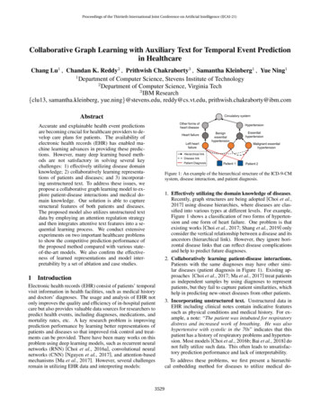
Proceedings of the Thirtieth International Joint Conference on Artificial Intelligence 5.3816.3322.5021.5323.58Table 5: R@k of predicting occurred/new-onset diseases.Without penaltyWith penalty.Patient had fairlyacutedecompensationofrespiratorystatustoday with hypoxia andhypercarbia associated withhypertension . Differential diagnosis includes flashpulmonary edema andacute exacerbation of CHFvs aspiration vs infection(HCAP) . Acuity suggestspossible flash pulmonaryedema vs aspiration .Patient had fairlyacutedecompensationof respiratory status today with hypoxia andassociatedhypercarbiawith hypertension . Differential diagnosis includesflash pulmonary edema andacute exacerbation of CHFvs aspiration vs infection(HCAP) . Acuity suggestspossible flash pulmonaryedema vs aspiration .Correct Predictions Hypertensive chronickidney disease Acute respiratory failure Congestive heart failure Diabetes .Table 6: An example of word contributions without/with the TFIDF rectified penalty. The pink/gray color denotes high/low attention weights.(a) GRAM level 1(b) GRAM level 2(c) GRAM level 3(d) Timeline level 1(e) Timeline level 2(f) Timeline level 3(g) CGL level 1(h) CGL level 2(i) CGL level 3Figure 3: Code embeddings in 3 levels learned by GRAM, Timeline,and CGL. Colors correspond to disease types in each level.diseases and the number of ground-truth diseases. We selectGRAM and MedGCN which have good performance in diagnosis prediction, and CGLn- without clinical notes, becausewe want to explore the effectiveness of the proposed observation and ontology graphs. Table 5 shows the results of R@kon test data. We can see that CGLn- has similar results toGRAM on occurred diseases while achieving superior performance on new-onset diseases. This verifies that our proposedcollaborative graph learning is able to learn from similar patients and predict new-onset diseases in the future.Disease embeddings. To show the similarity of diseases,we plot the learned 4795 code embeddings Hc using t-SNE[Maaten and Hinton, 2008]. Figure 3 shows the embeddingslearned by GRAM, Timeline, and CGL in 3 levels. Colorsdenotes different disease types in each level. In Figure 3, disease embeddings learned by GRAM and CGL are basicallyclu

c is the embedding matrix for nodes in level k, and d cis the embedding size. For a medical code c ias a leaf node, we first identify its ancestors in each level k [1;2;:::;K 1] in the tree and select corresponding embedding vectors from fE kg. Then, the hierarchical em-bedding e i 2RKd c of c iis calculated by concatenating the embeddings .