Transcription
Validation of a Web-Based Atmospheric Correction Tool for SingleThermal Band InstrumentsJulia A. Barsi*a, John R. Schottb, Frank D. Palluconic, Simon J. HookcaSSAI, NASA/GSFC Code 614.4, Greenbelt MD 20771Center for Imaging Science, RIT, Rochester NY 14623cNASA/JPL, MS 183-501, Pasadena CA 91109bABSTRACTAn atmospheric correction tool has been developed on a public access web site for the thermal band of the Landsat-5and Landsat-7 sensors. The Atmospheric Correction Parameter Calculator uses the National Centers for EnvironmentalPrediction (NCEP) modeled atmospheric global profiles interpolated to a particular date, time and location as input.Using MODTRAN radiative transfer code and a suite of integration algorithms, the site-specific atmospherictransmission, and upwelling and downwelling radiances are derived. These calculated parameters can be applied tosingle band thermal imagery from Landsat-5 Thematic Mapper (TM) or Landsat-7 Enhanced Thematic Mapper Plus(ETM ) to infer an at-surface kinetic temperature for every pixel in the scene.The derivation of the correction parameters is similar to the methods used by the independent Landsat calibrationvalidation teams at NASA/Jet Propulsion Laboratory and at Rochester Institute of Technology. This paper presents avalidation of the Atmospheric Correction Parameter Calculator by comparing the top-of-atmosphere temperaturespredicted by the two teams to those predicted by the Calculator. Initial comparisons between the predicted temperaturesshowed a systematic error of greater then 1.5K in the Calculator results. Modifications to the software have reduced thebias to less then 0.5 0.8K.Though not expected to perform quite as well globally, the tool provides a single integrated method of calculatingatmospheric transmission and upwelling and downwelling radiances that have historically been difficult to derive. Evenwith the uncertainties in the NCEP model, it is expected that the Calculator should predict atmospheric parameters thatallow apparent surface temperatures to be derived within 2K globally, where the surface emissivity is known and theatmosphere is relatively clear. The Calculator is available at http://atmcorr.gsfc.nasa.gov.Keywords: Landsat, Thematic Mapper (TM), Enhanced Thematic Mapper Plus (ETM ), thermal infrared (TIR),atmospheric correction1. INTRODUCTIONSince 1984, the systematic collection of Landsat imagery has produced more 60-120m high spatial resolution thermalinfrared (TIR) imagery of the Earth’s land surfaces than any other satellite system. Yet unlike other Earth observationmissions, the Landsat production system does not generate derived physical parameter products, such as sea surfacetemperature, from the calibrated at-satellite radiance data. The NASA/GSFC Land Cover Satellite Project ScienceOffice has developed a tool to allow the user to generate their own surface temperature products by calculating theeffects of the atmosphere for their site.The Atmospheric Correction Parameter Calculator has been on-line since 20031. Though the ancillary data and methodsare well known and used by the Landsat vicarious calibration teams, the automated tool has not been validated up to thispoint. This paper will discuss the Calculator and the validation of the Calculator over vicarious calibration sites.1.1 LandsatThe Thematic Mapper (TM) on the Landsat-5 satellite, launched March 1, 1984, and the Enhanced Thematic MapperPlus (ETM ) on the Landsat-7 satellite, launched April 15, 1999, each have a single 10.5-12.5µm TIR band2. Table I*julia.barsi@gsfc.nasa.gov; phone 1 301 614 6667; fax 1 301 614 6695Earth Observing Systems X, edited by James J. Butler, Proceedings of SPIE Vol. 5882 (SPIE, Bellingham, WA, 2005)0277-786X/05/ 15 · doi: 10.1117/12.619990Proc. of SPIE 58820E-1
1.2 Atmospheric CorrectionRemoving the effects of the atmosphere in the thermalregion is the essential step necessary to use the thermalband imagery for absolute temperature studies. Theemitted signal leaving a target on the ground is bothattenuated and enhanced by the atmosphere. Withappropriate knowledge of the atmosphere, a radiativetransfer model can be used to estimate the transmission,and upwelling and downwelling radiance. Once theseparameters are known, it is possible to convert theSpatialResolution(m)NE T(K at 280K)10.45 12.4210.31 12.361200.17 - 0.3060H: 0.22L: 0.28UsefulTemperatureRange(K)min: 230-330max: 200-340H: 240-320L: 130-350TABLE I.COMPARISON OF SELECTED FEATURES OF THE THERMALBANDS OF TM AND ETM . DUE TO THE BUILD UP OF ICE ON THELANDSAT-5 DEWAR WINDOW, THE LANDSAT-5 NOISE EQUIVALENTCHANGE IN TEMPERATURE IS SPECIFIED AS A RANGE. THE USEFULTEMPERATURE RANGE IS BOUNDED BY THE SENSITIVITY OF THEDETECTORS AT THE MINIMUM NE T AND THE RESCALING FACTORS FORTHE GEOMETRICALLY CORRECTED PRODUCT. LANDSAT-7 HAS NOTEXHIBITED ICING, BUT HAS TWO GAIN STATES SO THE SAME MEASRURESARE GIVEN SEPARATLY FOR HIHGH (H) NAD LOW (L) GAIN SETTINGS.(I/000000aJoUnlike multi-thermal band systems such as AVHRR,ATSR and ASTER, the Landsat instruments, each witha single thermal band, provide no opportunity toinherently correct for atmospheric effects. Ancillaryatmospheric data are required to make the correctionfrom Top-of-Atmosphere (TOA) radiance ortemperature to surface-leaving radiance or temperature.However, with the long history of calibrated data andthe current eight-day repeat cycle between the twoinstruments, there is strong motivation to use theseunique data for absolute temperature studies.Landsat-5TMLandsat-7ETM FWHM(µm)spectral responseprovides selected features of the thermal bands of thetwo instruments and the spectral response curves areshown in Figure 1. The calibration of TM thermal datahas not been rigorously monitored over its history,though a recent effort has shown data acquired since1999 may have a bias of –1.0K, though there may besome, as of yet, unresolved dependence on internalinstrument temperatures3.The ETM instrumentcalibration has been monitored since launch and iscalibrated to 0.6K at 300K4. The failure of the ScanLine Corrector (SLC) in 2003 does not appear to haveaffected the calibration of the thermal band.a 0.3O.2o.11/0II111213wavelength (!tm)TMLandsat-7 ETM space-reaching radiance to a surface-leaving radiance:Figure 1. Relative spectral response functions of the LandsatLTOA τεLT Lu τ (1 ε)Ld(1)thermal bands.where τ is the atmospheric transmission; ε is theemissivity of the surface, specific to the target type; LT is the radiance of a blackbody target of kinetic temperature T; Luis the upwelling or atmospheric path radiance; Ld is the downwelling or sky radiance; and LTOA is the space-reaching orTOA radiance measured by the instrument. Radiances are in units of W/m2·sr·µm and the transmission and emissivityare unitless. Radiance to temperature conversions can be made using the Planck equation or the Landsat specificestimate of the Planck curve:T k2 k ln 1 1 Lλ (2)where T is the temperature in Kelvin; Lλ is spectral radiance in W/m2·sr·µm; and k1 and k2 are calibration constantsgiven in Table II.Proc. of SPIE 58820E-2
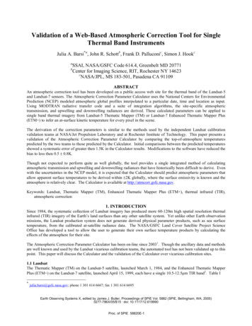
The radiance measured at the satellite can be converted to a TOAtemperature. However, TOA temperature is not a good estimateof surface temperature. Neglecting the atmospheric correctionwill result in systematic errors in the predicted surface temperaturefor any given atmosphere. Figure 2 illustrates the errors in surfacetemperature if no atmospheric correction is made for a series of thevicarious calibration scenes, i.e. if the TOA temperature is used asthe surface temperature. For a single day, the temperature will besystematically off, but the error will be different for different daysbased on the properties of the atmosphere at the overpass .76Landsat-7 ETM Landsat-5 TMTABLE II. THERMAL BAND CALIBRATION CONSTANTS TOCONVERT RADIANCE TO TEMPERATUREAI2. ATMOSPHERIC CORRECTION PARAMETERCALCULATORTraditionally, calculating the atmospheric transmission andupwelling radiance has been difficult and time consuming. Theuser has to know where to get the atmospheric data, convert it tothe proper format for a radiative transfer model and integrate theresults over the proper band pass. The Atmospheric CorrectionParameter Calculator facilitates this calculation.2.1 The Web-Based ToolThe Calculator requires a specific date, time and location as input(Figure 3). It outputs the parameters the user will need to convertthe satellite radiance to surface radiance. The user has the optionto select the TM bandpass, the ETM bandpass, or no spectralbandpass, in which case, only the atmospheric profiles are output.Another option allows the user to select how the modeledatmospheric profile is interpolated. If local surface conditions areavailable, the user can enter them. The local conditions will beused instead of the surface layer predicted by the model, and thelower layers of the atmosphere will be interpolated from 3kmabove sea level to the surface to remove any discontinuities. Arecently added option is the choice between the summer standardatmosphere and the winter standard atmosphere for the upperlayers.Fb 03Ag 03 D 03 M 04My 0306t 04Figure 2. Difference between measured surfacetemperature and predicted TOA temperature for twoyears and two sites. If the TOA temperature wereused as surface temperature, the temperatureestimate would be incorrect by the difference shownhere.Year:Month:Lattude: flflDay:Minute: n nttMT Hour:Lornyltude: flflo Use aumosplnerlc profile for closest Irdeger laVlorng youUse Interpolated atmospherIc profile for gIven laViong toto Use mld-lattudesummerstandard atmosphere for upper atmospherIc profile yetUse mid-lattude winter standard atmosphere for upper atmospherIc profile yetS Use Landyat-7 Band sal rosnse curseo Use Landsat-5 Band sal rosnse curseo OLutput only atirosplner:c profile, do ret calculate effectve radlancesOpuonal: Surface CoedItorsAlttude (her): flflTemperature (C):The calculated results are emailed to the user and output to theweb browser. The emailed file contains not only the integratedtransmission and up- and downwelling radiances for the given site,but also all the atmospheric data used to generate the results. Inthe case where no spectral bandpass is selected, the output is theinterpolated atmospheric profiles, for use in a radiative transfermodel.J 04ig qiiti dt Ldt5JPL2003ALdt7RI 2004Pressure (mb):Relatse HumIdIty (fit): IIResults will be sent to the followIng address:Figure 3. The Atmospheric Correction ParameterCalculator web interface.The atmospheric profiles are generated by the National Centers for Environmental Prediction (NCEP). Theyincorporate satellite and surface data to predict a global atmosphere at 28 altitudes. These modeled profiles are sampledon a 1 x1 grid and are generated every six hours, 00:00, 06:00, 12:00, and 18:00 GMT. The Calculator provides twomethods of resampling the grid for the specific site input: “Use atmospheric profile for closest integer lat/long” or “Useinterpolated atmospheric profile for given lat/long”. The first extracts the grid corner that is closest to the location inputfor the two time samples bounding the time input and interpolates between the two time samples to the given time(Figure 4a). The second option extracts the profiles for the four grid corners surrounding the location input before andProc. of SPIE 58820E-3
after the time input (Figure 4b). The corner profiles areinterpolated for each time, then the resulting timeprofiles are interpolated resulting in a single profile.The location and time-specific interpolated profilecontains pressure, air temperature and water vaporprofiles from the surface to about 30km above sea level.In order to predict space-reaching transmission andupwelling radiance, the radiative transfer code,MODTRAN, requires profiles reaching “space”, or100km above sea level. Either the MODTRAN midlatitude summer or mid-latitude winter standardatmospheres are extracted from a MODTRAN standardatmosphere and the upper atmospheric layers ( 30100km) pasted onto the site specific interpolated profile.This results in a surface-to-space profile for airtemperature, water vapor and pressure.-I—,timeThe completed profile is inserted into a MODTRAN 4.0input file and processed. The spectral transmission andupwelling radiance are extracted from the MODTRANoutput files and integrated over the appropriateinstrument’s bandpass. The downwelling radiance isgenerated by running MODTRAN again, placing theIsensor 1m above a target with unit reflectance. The timesurface radiance in the new MODTRAN output file isFigure 4. The two interpolation methods. In (a), the profilestaken to be the spectral downwelling radiance and isare only interpolated in time, In (b), the profiles areintegrated over the instrument bandpass.interpolated in both space and time. The resulting integrated transmission, upwelling and downwelling radiance are output to the browser and emailed to theuser for use in removing the effects of the atmosphere with Equation (1), where the emissivity is specific to each surfacetype. The Atmospheric Correction Parameter Calculator is located at http://atmcorr.gsfc.nasa.gov.2.2 ValidationWhile techniques the Calculator makes use of have been tested, the Calculator has been in use for several years withoutvalidation. The Landsat vicarious calibration teams at NASA/Jet Propulsion Laboratory (JPL) and Rochester Instituteof Technology (RIT) have their own versions of an atmospheric correction routine5,6. While the Calculator borrowsheavily from both the RIT method and the JPL atmospheric data, the results of their algorithms had not previously beencompared to those of the web-based Calculator.JPL has installed an automated buoy system on Lake Tahoe, California. RIT takes ground truth on Lakes Ontario andErie. Both teams measure the surface temperature or radiance of their target, a large isothermal body of water. Usingtheir atmospheric correction method, they each predict a TOA radiance for their targets. The calibration processinvolves comparing their predicted TOA radiance to the radiance measured by the Landsat instrument. The two TOAradiances should match, within the error of the process. In the validation of the Atmospheric Correction ParameterCalculator, the Landsat measured radiance is ignored. The TOA predictions of the ground teams are taken as truth.The dates and locations for two years of vicarious calibration efforts were input into the Calculator. The JPLcomparison was made for Landsat-5 2003 data; the RIT comparison for Landsat-7 2004 data. The JPL site is a uniquecalibration target: the high altitude of Lake Tahoe means the atmosphere is generally clear and the atmospheric path istwo kilometers shorter then for surfaces closer to sea level. The lake also is positioned on an integer latitude/longitudeProc. of SPIE 58820E-4
(39/-120) and the Landsat-5 overpass time is at approximately18:15GMT in 2003, so the Calculator is essentially using asingle entry from the NCEP database. The RIT site is closerto what the general user will encounter: it is not on oneof the integer latitude/longitude corners (43.26/-77.56) and theLandsat-7 data is acquired at about 15:40GMT in 2004 nearlymidway between NCEP time samples.In the initial validation effort, the data were systematicallyover corrected, i.e. the TOA temperature was too cold. ForJPL, the error was on the order of 1.5K; for RIT, the error wasabout 2.5K. The large day-to-day variation was corrected for,but a systematic error remained.An error was found in the calculation of band averagetransmission. This caused a 3% error in the estimation of thetransmission.The band pass over which the spectraltransmission was averaged was too wide; it extended beyondthe wavelengths where the instrument was actually sensitive.This was corrected by limiting the average to the wavelengthsbetween the full-width, half maxima of the instrument’sspectral response curve.The difference in calculatedtransmission for the JPL Landsat-5 2003 data was a constant0.03; for RIT Landsat-7 2004 it was between 0.03 and 0.05.This error appears to have caused most of the error betweenthe TOA temperatures predicted by JPL and RIT and thosepredicted using the Calculator’s parameters. The correctionwas implemented on June 22, 2005.There is still a systematic bias between the new Calculatorpredicted TOA temperatures and those of JPL and RIT, but itis much smaller. Figure 5 and Table III show the difference inTOA predicted temperatures between the JPL or RITpredicted TOA temperature and the Calculator-based TOApredicted temperature (TTOA(AtmCorr)). The average bias isless then -0.5K (Table IV), though after adjusting for the sitespecific bias, the RMS for the two sites are different, 0.22Kfor Lake Tahoe and 0.76K for Lake Ontario. The final threedates from the RIT set all have low transmissions and largererrors. There is some evidence that the NCEP profiles don’twork as well when the column water vapor total is above 2.0cm7, which may be the problem on the low transmissiondates, though this has not been tested in the validation yet.The difference in the RMS error could just be related to theidealized conditions at Lake Tahoe or there could be adifference in the way the two band passes should be p-04Landsat-5 JPL2003Landsat-7 53-0.78-0.27-0.44-0.33-0.16-1.54-0.631.03TABLE III. CALCULATED DIFFERENCE IN TOA TEMPERATURE(RIT OR JPL-ATMCORR). THE DATES WHEN THE TRANSMISSIONIS LESS THEN 0.85 ARE SHADED IN THE TABLE.0.5I.Fel -03 May-03.Aug-03Dec-03Mar-04 Jun-04Oc -04A0acquisition date Landsat-5 JPL 2003 with surf ace correction A Landsat-7 RIT 2004 with surf ace correctionFigure 5. The date-average difference between the JPL orRIT predicted TOA temperature and the Calculatorpredicted temperature. The dates with transmission lessthen 0.85 are hollow.Landsat-5 JPL 2003Landsat-7 RIT 2004residual error[K]-0.48-0.31RMS [K]0.220.76TABLE IV. VALIDATION RESULTS FOR THE TWO SITESThese results presented here were calculated using atmospheres which have been corrected for local surface conditions.Although there was no statistical difference between the TOA temperatures calculated using the model surfaceconditions and the local surface conditions, it is believed that the local surface conditions should help generate a betterprediction. In all of these cases, the model surface was several tenths of kilometers above where the surface actually is,probably due the location of the weather stations. For example, in Rochester, NY, weather is recorded at the airportwhich is at a higher altitude above sea level then the Lake Ontario shoreline. This lowest portion of the atmosphere isProc. of SPIE 58820E-5
typically the thickest so neglecting even a small amount should affect the prediction of the atmospheric parameters.However, for these dates, although entering the surface conditions did not have obvious benefit, it also did no harm.Several other minor changes were made during the validation effort: The interpolation altitude when surface layers are input was changed from 5km to 3km. A sort was added to the atmospheric layers to ensure they were in proper order, lowest to highest altitude. Theinterpolation of the four corners based on the pressure levels resulted in some cases where the first layer in theprofile was not the lowest altitude.2.3 Limitations The Calculator generates parameters for a single point. In some cases, this may be adequate to describe theatmosphere across a whole scene. In others, especially where there is considerable elevation change, morethen one run of the Calculator may be necessary to characterize the atmosphere over the scene. There is no automatic check for clouds or discontinuities in the interpolated atmosphere. The user shouldcheck the profiles contained in the emailed summary file for problems. At present, however, there are no plansto add the ability to modify such a problem atmosphere. The user must know the emissivity of the target in order to calculate LT. A library of spectral emissivities ofmany target types is available at http://speclib.jpl.nasa.gov. NCEP data, in the format currently used, are not available for the entire lifetime of Landsat-7 or Landsat-5.The NCEP holdings include all dates since March 1, 2000. The interpolation in time and space is linear. This may not be the most appropriate method for samplingweather fronts or the diurnal heating cycle.2.4 Future Efforts The remaining systematic error needs to be reduced. More validation data, including the RIT Landsat-5 data,can be used to track down the bias. This will also help establish whether the NCEP atmospheres are reliable inwetter conditions. The method being used to calculate downwelling radiance should be validated against a full hemisphere raytrace method. The bandpass average transmission should be calculated using the ratio of radiances of targets of differenttemperatures, rather then band average of the predicted spectral transmission. Atmospheric data is available for the entire lifetime of Landsat-5, but it is in a different format. The interfaceneeds to be developed to extract the atmospheric profiles from the file format that is available for those yearsthat are not yet available. With this effort, the tool could be useful for Landsat-4 data as well.3. CONCLUSIONSWith the abundance of Landsat data now available at low cost and without restrictions on distribution, it is important tomake the archive of at-satellite thermal data as usable as possible. The Atmospheric Correction Parameter Calculatorprovides an automated method to derive atmospheric correction parameters needed for generating surface temperatures.Initial validation efforts revealed a systematic error of greater then 1.5K. Corrections have reduced the bias to less the0.5 0.8K. Work will continue to remove the remaining bias entirely.Landsat-5 and Landsat-7 data are available from the USGS National Center for Earth Resources Observation andScience (EROS) at http://earthexplorer.usgs.gov and http://glovis.usgs.gov. The Atmospheric Correction ParameterCalculator is available at s to the Landsat vicarious calibration teams at Rochester Institute of Technology and NASA/Jet PropulsionLaboratory for use of their data and methods.REFERENCES1.Barsi, J.A., J.L. Barker, J.R. Schott. “An Atmospheric Correction Parameter Calculator for a Single Thermal BandEarth-Sensing Instrument.” IGARSS03, 21-25 July 2003, Centre de Congres Pierre Baudis, Toulouse, France.Proc. of SPIE 58820E-6
2.3.4.5.6.7.Markham, BL., Storey, J.C., Williams, D.L., Irons, J.R., “Landsat Sensor Performance: History and Current Status”IEEE Transactions on Geoscience and Remote Sensing, 42, pp. 2810-2820, 2004.Barsi, J.A., G. Chander, B.L. Markham, N.J. Higgs, “Landsat-4 and Landsat-5 Thematic Mapper Band 6 Historicalperformance and calibration.” Proceedings of Earth Observing Systems X, (this issue), SPIE, Bellingham, WA,2005.Barsi, J.A., J.R. Schott, F.D. Palluconi, D.L. Helder, S.J. Hook, B.L. Markham, G. Chander, E.M. O’Donnell,“Landsat TM and ETM Thermal Band Calibration,” Canadian Journal of Remote Sensing. 28, pp. 141-153, 2003.J. R. Schott, J. A. Barsi, B. L. Nordgren, N. G. Raqueno, and D. de Alwis. “Calibration of Landsat thermal dataand application to water resource studies,” Remote Sensing of Environment, 78, pp 108-117, 2001.Hook SJ, Chander G, Barsi JA, Alley RE, Abtahi A, Palluconi FD, Markham BL, Richards RC, Schladow SG,Helder DL. “In-flight validation and recovery of water surface temperature with Landsat-5 thermal infrared datausing an automated high-altitude lake validation site at Lake Tahoe” IEEE Transactions on Geoscience and RemoteSensing, 42, pp. 2767-2776, 2004.F. D. Palluconi, personal communicationProc. of SPIE 58820E-7
spectral response 000000 ajo / (i a 0.3 o.2 o.1 0 1/ i i 11 12 13 wavelength (!tm) tm landsat-7 etm table i. comparison of selected features of the thermal bands of tm and etm .due to the build up of ice on the landsat-5 dewar window, the landsat-5 noise equivalent change in temperature is specified as a range.the useful temperature range is bounded by the sensitivity of the