Transcription
Evolutionary Computation Applied to the Tuningof MEMS GyroscopesDidier Keymeulen, Wolfgang Fink, Michael I. Ferguson, Chris Peay, Boris Oks,Richard Terrile, and Karl YeeJet Propulsion LaboratoryCalifornia Institute of TechnologyPasadena, CA 91109, USA 1 (818) 354-4280didier.keymeulen@jpl.nasa.govsprings. Because of the time consuming nature of the tuning processwhen performed manually, in practice any set of bias voltages thatproduce degeneracy is viewed as acceptable at the present time. Aneed exists for reducing the time necessary for performing thetuning operation, and for finding the optimally tuned configuration,which employs the minimal maximum tuning voltage.This paper describes the application of evolutionarycomputation to this optimization problems. Evolutionarycomputation was first introduced by John Holland in USA [5] andRechenberg [11] and Schwefel [12] in Europe to solve optimizationproblems. Our method used as a fitness function for each set of biasvoltages applied to built-in tuning pads, the evaluation of thefrequency split between the two modes of resonance of the MEMSgyroscope. Our evaluation proceeds in two steps. First, it measuresthe frequency response using a dynamic signal analyzer. Second, itevaluates the frequency of resonance of both modes by fittingLorentzian curves to the experimental data. The process of settingthe bias voltages and the evaluation of the frequency split iscompletely computer automated. The computer controls a signalanalyzer and power supplies through General Purpose Interface Bus(GPIB). Our method has demonstrated that we can obtain afrequency split of 52mHz in one hour compared with 200mHzobtained manually by humans in several hours.ABSTRACT1We propose a tuning method for MEMS gyroscopes based onevolutionary computation to efficiently increase the sensitivity ofMEMS gyroscopes through tuning and, furthermore, to find theoptimally tuned configuration for this state of increased sensitivity.The tuning method was tested for the second generation JPL/BoeingPost-resonator MEMS gyroscope using the measurement of thefrequency response of the MEMS device in open-loop operation.Categories & Subject Descriptors: B.6.3 VerilogGeneral Terms: AlgorithmsKeywordsGenetic Algorithms, Simulated Annealing, Dynamic Hill Climbing,Evolvable Hardware, Gyroscope, MEMS.1. INTRODUCTIONFuture NASA missions would benefit tremendously from aninexpensive, navigation grade, miniaturized inertial measurementunit (IMU), which surpasses the current state-of-the art inperformance, compactness and power efficiency. Towards this end,under current development at JPL’s MEMS Technology Group areseveral different designs for high performance, small mass andvolume, low power MEMS gyroscopes. The accuracy with whichthe rate of rotation of micro-gyros can be determined dependscrucially on the properties of the resonant structure. It is expensiveto attempt to achieve these desired characteristics in the fabricationprocess, especially in the case of small MEMS structures, and thusone has limited overall sensor performance.The sensitivity of the MEMS gyroscope is maximized whenthe resonant frequencies of the two modes of freedom of a MEMSgyroscope are identical. Symmetry of construction is necessary toattain this degeneracy. However, despite a symmetric design, perfectdegeneracy is never attained in practice. Tuning of the gyros into thestate of degeneracy is achieved through application of bias voltageson built-in tuning pads to electrostatically soften the mechanical2. TEST SETUP FOR GYRO TUNINGTwo stochastic optimization methods based on evolutionarycomputation, namely dynamic hill climbing and simulated annealingalgorithms, have been implemented on a dedicated, JPL/Boeingspecific hardware platform, which is described in the followingsections.2.1 Mechanism of the JPL MEMS Micro-gyroThe mechanical design of the JPL MEMS microgyro can beseen in Figure 1. The JPL/Boeing MEMS post resonator gyroscope(PRG), is a MEMS analogue to the classical Foucault pendulum. Apyrex post, anodically bonded to a silicon plate, is driven into arocking mode along an axis (labeled as X in Figure 1) by sinusoidalactuation via electrodes beneath the plate. In a rotating referenceframe the post is coupled to the Coriolis force, which exerts atangential “force” on the post. Another set of electrodes beneath thedevice senses this component of motion along an axis (labeled as Yin the figure) perpendicular to the driven motion. The voltage that isrequired to null out this motion is directly proportional to the rate ofrotation to which the device is subjected. A change in capacitanceoccurs as the top plate vibrates due to the oscillating gap variationCopyright 2005 Association for Computing Machinery. ACM acknowledges that this contribution was authored or co-authored by a contractoror affiliate of the U.S. Government. As such, the Government retains anonexclusive, royalty-free right to publish or reproduce this article, or toallow others to do so, for Government purposes only.GECCO’05, June 25–29, 2005, Washington, DC, USA.Copyright 2005 ACM 1-59593-010-8/05/0006 5.00.927
The frequency split reduces the mechanical coupling betweenthe two modal axes, and thus reduces the sensitivity for detection ofrotation. By adjusting the static bias voltages on the capacitor plates,frequencies of resonance for both modes are modified to match eachother; this is referred to as the tuning of the device.In order to extract the resonant frequencies of the vibrationmodes, there are two general methods: 1) open-loop and 2) closedloop control [9]. In an open-loop system, we are measuring thefrequency response along the drive axis over a 50Hz band andextract from the measurement the frequency split. A faster method isa closed-loop control, whereby the gyro is given an impulsedisturbance and is allowed to oscillate freely between the tworesonance frequencies, using a hardware platform, controlling theswitch of the drive-angles [10].between this plate and the electrodes underneath. This change incapacitance generates a time-varying sinusoidal charge that can beconverted to a voltage using the relationship V Q/C. The post canbe driven around the drive axis by applying a time-varying voltagesignal to the drive petal electrodes labeled D1-, D1 , D1in- andD1in in Figure 1. Because there is symmetry in the device, eitherof the two axes can be designated as the drive axis. Each axis has acapacitive petal for sensing oscillations as well; driving axis: labeledS1 and S1- in Figure 1, sensing axis: labeled S2 and S2- in Figure1. The micro-gyro has additional plates that allow for electro-staticsoftening of the silicon springs, labeled B1, BT1, B2, and BT2 inFigure 1. Static bias voltages can be used to modify the amount ofsoftening for each oscillation mode. In an ideal, symmetric device,the resonant frequencies of both modes are equal; however,unavoidable manufacturing imperfections in the machining of thedevice can cause asymmetries in the silicon structure of the devices,resulting in a frequency split between the resonant frequencies ofthese two modes.The measurement consists of exciting the drive axis with a sinewave at a given frequency and measuring the resulting amplitude.This is done repeatedly through the frequency spectrum. Because ofcross-coupling between the different axes, two peaks in theamplitude response will appear at two different frequencies,showing the resonant frequencies of both axes (Figure 7). This takesapproximately 1.4 minutes to complete using our instrumentationplatform and must be done at least three times to average out noise.ZΩXθ1Y2.2 Instrumentation PlatformThe platform includes one GPIB programmable power supplyDC voltage, a GPIB signal analyzer to extract frequency responses(from 3.3kHz to 3.35kHz) of the gyro in open-loop, and a computer(PC) to control the instruments and execute the optimizationalgorithms. The power supply DC voltage controls the static biasvoltages (connected to the plate B1, BT1, B2, and BT2 in Figure 1)that are used to modify the amount of damping to each oscillationmode. The GPIB signal analyzer generates a sine wave with avariable frequency (from 3300 Hz to 3350 Hz and a step of 62.5mHz – 800 points, 50Hz span) on the drive electrode (D1-, D1 ,D1in- and D1in in Figure 1) and measures the response signal onthe sense electrode (S1-, S1 in Figure 1) along the drive axis X.A PC runs the instrument control tool, the measurement tool,and the evolutionary computation tool. The instrument controlsoftware sets up the static bias voltages using the GPIB powersupply DC voltage and measures the frequency response along theX axis using the GPIB signal analyzer as shown in Figure 2. Themeasurement tool software calculates the frequency split using peakfitting algorithms. Finally the evolutionary computation toolsoftware determines the new DC bias voltages from the frequencysplit. This procedure is repeated until a satisfactory frequency split isobtained.θ2XYFigure 1. A magnified picture of the JPL MEMS microgyroscope with sense axis Y (S2-, S2 electrodes used to sense,D2-, D2 , D2in- and D2in used to drive along the sense axis)and drive axis X (D1-, D1 , D1in- and D1in used to drive, S1-,S1 electrodes used to sense along the drive axis) and theelectrodes used for biasing (B1, B2, BT1, BT2) (picture courtesyof C. Peay, JPL).928
void SetupStimulus (float startF ,float span )EvolutionaryGeneticAlgorithmsAlgorithmwhich are time expensive, the results of all evaluations are cached. Ifthe found optimum is of an un-acceptable fitness, a new startingpoint is found by computing the location that is farthest in the searchspace from all known local optima. The step size is set at a value of10 volts and we repeat the process until a desired optimum is found.void SetupDC (float B1, float BT1,float B2,voidfloat BT2)Init Instruments ()Option1:void GetResponse (float * f1, float * f2, float *f1a, float * f2a)[minimize abs(f1-f2), maybe use f 1a and f2a(amplitude) information ]Option2: void GetResponse (float * f split)[minimize f split]AGT35670AAnalyzer(2 channel)Stimulus 1,2 (τ)Response 1,2 (θ)3.2 Simulated Annealing AlgorithmsSimulated annealing (SA) is a widely used and high-dimensionalconfiguration spaces [7, 8]. The goal is to minimize an energyfunction E, akin to the fitness function used in GAs, which is afunction of N variables, with N being usually a large number. In ourcase, the energy function is the frequency split of the MEMS microgyroscope, and N 4 is the number of the bias voltages Theminimization is performed by randomly changing the value of oneof the 4 bias voltages and reevaluating the energy function E, i.e.,the resulting frequency split. Two cases can occur: 1) the change inthe bias voltage results in a new, smaller frequency split; or 2) theresulting frequency split is larger or unchanged. In the first scenariothe new set of bias voltages is stored and the change accepted. In thesecond scenario, the new set of bias voltages is only stored with acertain likelihood (Boltzmann probability, including an annealingtemperature). This ensures that the overall optimization algorithmdoes not “get stuck” in local minima too easily, as is the case withgreedy downhill optimization, and hence to fail to find the desiredglobal minimum. The annealing temperature directly influences theBoltzmann probability by making it less likely to accept anenergetically unfavorable step, the longer the optimization lasts(cooling schedule). Then the overall procedure is repeated until theannealing temperature has reached its end value, or a preset numberof iterations has been exceeded, or the energy function E, i.e., thefrequency split, has reached an acceptable level. In contrast tostandard simulated annealing, we apply a modified simulatedannealing related algorithm, in which the annealing temperatureoscillates between to boundaries (reheating / recooling), with thelower boundary being a fixed, small value 0 and the upperboundary being the current best frequency split. The exit criterion inour case is the reaching of a desired minimal frequency split.DC PowerSuppliesGyroB1, B2, BT1, BT2Figure 2. Software interface between the SimulatedAnnealing/Modified Genetic Algorithm and the InstrumentationPlatform using a GPIB programmable power supply DC voltageand a signal analyzer. The Simulated Annealing and GA/HillClimbing are running on a PC, which controls the bias voltagesand receives the frequencies of both resonance modes.3. OVERVIEW OF ALGORITHMSAs with most prototype sensor development efforts, theJPL/Boeing MEMS post-resonator gyroscope is custom-built andhand-tuned for optimal performance. Many methods have beendeveloped for tuning MEMS post-resonator gyroscopes. Forexample [1] and [2] use adaptive and closed-loop methods while [3]changes the frame of the pick-off signal. As explained in Section 2,our approach of gyro tuning consists of adjusting 4 bias voltagesbetween -60V and 14V on capacitor plates to reduce the frequencysplit. Our approach can be seen as an optimization problem wherethe value to minimize is the difference between two frequencies andthe parameters are the four bias voltages. We propose two stochasticoptimization algorithms – dynamic hill climbing and simulatedannealing used for different space applications [4], to optimize thevalues of bias voltages applied to built-in tuning pads on the MEMSpost-resonator gyroscope.4. EVALUATION OF THE FREQUENCYSPLIT3.1 Dynamic Hill Climbing AlgorithmWe have developed a method to extract the peak from thefrequency response using a peak fitting algorithm based on amodel of the transfer function of the MEMS micro-gyro [9].The transfer function H(s) for a single input- single output(SISO) system, modeling the gyro behavior, is described inEquation 1. The transfer function relates the angle velocity ofTo reduce the number of evaluations of potential solutions weused a Dynamic Hill Climbing introduced by Yuret et al. [6]. Westart with a potential solution represented by a point in a fourdimensional search space that is easiest to implement (from thehardware standpoint). Our initial point is obtained by setting thestatic bias voltages (connected to the plate B1, BT1, B2, and BT2 inFigure 1) to [ 14Volt] [ 14Volt] [ 14Volt] [ 14Volt]. It istherefore setting the potential between the bias plates and thecommon plate to zero since the common plate is held 14 volts. Wethen use a hill climbing method to find the best neighboring point.In our four dimensional space we examine eight neighboring points( /- step size in each dimension, one dimension at a time). Originalvalue of step size is 10 volts. Once an optimum point is found withthe original step size (no neighboring points give a higher fitness),the step size is halved and the hill climbing is restarted using the halfstep size. The step size is continually halved until it is equal to 0.1volts, we accept the optimum at this point and the location of thisoptimum is saved. To avoid multiple evaluations of the same pointsthe drive axesθ&1and the torque in the drive axesτ 1 . Theconstants in the equation are as follows: ω d : natural resonance of the sensor axis’ driving mode Qd : quality factor depends on the spring constantJ t : symmetric moments of inertia around the X and Y axes H (S ) 929( 1J ) SωdS2 (t2Qd ) S ω d(1)
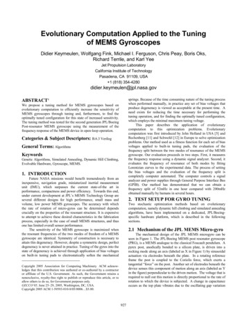
calculated/Lorentzian model. The Chi Squared is calculated asfollows:The SISO model is approximated by the Lorentzian functionshown in Equation 2 and illustrated in Figure 3. It ischaracterized by having a very sharp and narrow peak withmost of the intensity of the peak located in the tails (or“wings”), extending to infinity (Figure 3).f ( x) Hx x4( w 0 )2 1nχ 2i Calculatedi )2 ( ActualRMSNoisei 0n f(3)where RMSNoise is the estimated Root Mean Squared noise inthe actual data. The variable n is the number of data points and f isthe total number of variables in the Lorentzian model, i.e., 6.(2)where X0 Peak Position, H Peak Height, W Full widthat Half Height.The process of optimizing the 6 parameters in the Lorentzianmodel is described below:Start at default values for all 6 variables.Fixed an initial value for the step sizeLoop until step size threshold1.Vary L1 and L2 by one step size while keeping allother parameters at their best values, calculate theLorentzian model and evaluate the Chi2 of the fittestcurvesa.Figure 3. Lorentzian functions with different values used toapproximate the transfer function of a SISO system, modelingthe MEMS micro-gyro behavior.2.The objective is to fit the sum of two Lorentzian functions tothe frequency response experimental data as illustrated in Figure 4.We can then calculate the frequency split between the two modes ofresonance by measuring the difference of the peak locations of eachLorentzian function.Vary H1 and H2 one step size while using bestparameters obtained so far, calculate the Lorentzianmodel and evaluate the Chi2 of the fittest curves.a.3.Split 1.5648 HzAmplitude of Oscillation (arbitrary units)35Save values of W1 and W2 that producelowest Chi2Save the set of variable L1, L2, H1, H2, W1, W2 giving the bestChi2.30If the variation of Chi2 from previous iteration is equal to zerothen decrease step size2520Once all six parameters are determined, the frequency split isfound by taking the difference between L1 and L2.155. RESULTS OF EVOLUTIONARYCOMPUTATION1050Save values of H1 and H2 that producelowest Chi2Vary W1 and W2 one step size while using bestparameters obtained so far, calculate the Lorentzianmodel and evaluate the Chi2 of the fittest curves.a.Lorentzian FitSave values of L1 and L2 that producelowest Chi233213322332333243325Frequency (Hz)3326The MEMS post resonator micro-gyroscope, developed by theMEMS Technology Group at JPL, is subject to an electro-staticfine-tuning procedure, performed by hand, which is necessary due tounavoidable manufacturing inaccuracies. In order to fine-tune thegyro, 4 voltages applied to 8 capacitor plates have to be determinedwithin a range of –60V to 15V, respectively. The manual handtuning took several hours and obtained a frequency split of 200mHz.In order to fully automate the time-taking manual fine-tuningprocess, we have established a hardware/software interface to theexisting manual gyro-tuning hardware-setup using commercial-offthe-shelf (COTS) components described in Section 4.We developed and implemented two stochastic optimizationtechniques for efficiently determining the optimal tuning voltagesand incorporated them in the hardware/software interface: amodified simulated annealing related algorithm and a modifiedgenetic algorithm with limited evaluation.3327Figure 4. Fitting the sum of two Lorentzian functions to thefrequency response experimental data. The green and bluecurves are Lorentzian functions and the red curve is the sum ofthe two functions. The experimental data points are plotted inblack.Each Lorentzian function is completely described by 3parameters as shown in Equation 2. To come up with twoLorentzian functions, the sum of which best describes theexperimental data, we have to optimize a total of 6 parameters.Lorentzian 1: location (L1), width (W1), height (H1)Lorentzian 2: location (L2), width (W2), height (H2)We have used the Chi Square statistic to measure theagreement between actual/experimental/measured data and930
5.1 Simulated Annealing ApproachFrequency Split vs. Number of EvaluationsWe were able to successfully fine-tune both MEMS postresonator gyroscope and MEMS disk-resonating gyroscope (adifferent gyro-design not discussed here) within one hour for thefirst time fully automatically. After only 49 iterations with themodified Simulated Annealing related optimization algorithm weobtained a frequency split of 125mHz within a 1V-discretization ofthe search space, starting with an initial split of 2.625Hz, using a50Hz span and 800 points on the signal analyzer for the MEMSpost-resonator gyroscope (Figure 5 top). For the MEMS diskresonating-gyroscope we obtained a frequency split of250mHz/500mHz within a 0.1V-/0.01V-discretization of the searchspace, starting with an initial split of 16.125Hz/16.25Hz, after249/12 iterations using a 200Hz span and 800 points on the signalanalyzer (Figure 5 bottom). All three results are better than what canbe accomplished manually but worse than the results obtained bydynamic hill climbing. The results can be further improved, usingthe peak fitting algorithm employed in the dynamic hill climbingapproach.1.6Frequency Split (Hz)1.41.210.80.60.40.2001020304050Number of EvaluationsFigure 6. Frequency split as a function of number of evaluationsused by the Dynamic Hill Climbing algorithm.Lorentzian FitAmplitude of Oscillation (arbitrary units)40Split 1.5648 HzExperimental DataL1L2Combination L1 L23020100-10-20-30-40-503300331033203330Frequency (Hz)Lorentzian Fit33403350Split 1.5648 HzAmplitude of Oscillation (arbitrary units)3530252015105033213322332333243325Frequency (Hz)33263327Figure 7. Frequency response (top: 50Hz band, bottom: 6Hzband) before tuning using the modified genetic algorithm. Thefrequency split is 1555mHz. The Y axis is measured in dB. Theinitial values of the four bias voltages are: B1 14.00V BT1 14.00V B2 14.00V BT2 14.00V. The bottom picture shows azoom of the frequency split over a 6Hz band.Figure 5. Frequency split as a function of Simulated AnnealingIterations: (top) for the MEMS post-resonator gyroscope;(bottom) for the MEMS disk-resonating gyroscope.5.2 Modified Genetic Algorithm ApproachWe were also able to fine-tune the MEMS post-resonatorgyroscope within one hour fully automatically using a geneticrelated algorithm: dynamic hill climbing. Figure 6 shows theprogress of the optimization algorithm aimed at minimizing thefrequency split. Each evaluation is a proposed set of bias voltages.Our optimization method only needed 47 evaluations (51 min) toarrive at a set of bias voltages that produced a frequency split of lessthan 100mHz.Figures 7 and 8 show the frequency response for the unbiasedmicro-gyro respectively before and after tuning using the dynamichill climbing and the peak fitting algorithm.After optimization of the bias voltages (Figure 8), thefrequency split has been minimized to less than 100mHz and thetwo peaks are indistinguishable on an HP spectrum analyzer at62.5mHz / division (50Hz span, 800 points) setting, which was usedduring the optimization process.931
Amplitude of Oscillation (arbitrary units)50Lorentzian Fit7. ACKNOWLEDGMENTSSplit 0.05237 HzThe work described in this publication was carried out at the JetPropulsion Laboratory, California Institute of Technology, under acontract with the National Aeronautics and Space Administration.Special thanks to Tom Prince, who has supported this researchthrough the Research and Technology Development grant entitled“Evolutionary Computation Technologies for Space Systems” andto Thomas George, head of the MEMS Technology Group at JPL,who has encouraged the research from its beginning.Experimental DataL1L2Combination L1 L2403020100-10-208. REFERENCES-30[1] Leland, R.P., “Adaptive mode tuning vibrational gyroscopes”,IEEE Trans. Control Systems Tech., vol. 11, no. 2, pp242-247,March 2003.-40-503300331033203330Frequency (Hz)Amplitude of Oscillation (arbitrary units)Lorentzian Fit33403350[2] Painer C.C., Shkel A.M., “Active structural error suppressionin MEMS vibratory rate integrating gyroscopes”, IEEE SensorsJournal, vol.3, no.5, pp. 595-606, Oct. 2003.Split 0.05237 Hz[3] Y. Chen, R. M’Closkey, T. Tran and B. Blaes. “A control andsignal processing integrated circuit for the JPL-Boeingmicromachined gyroscopes” (submitted to IEEE)4035[4] R. J. Terrile, et al., “Evolutionary Computation Technologiesfor Space Systems”, in Proceedings of the IEEE AerospaceConference, Big Sky, March 20053025[5]J.H. Holland, Adaptation in Natural and Artificial Systems,The University of Michigan Press, Ann Arbor, Michigan,1975.[6]D. Yuret, M. de la Maza, “Dynamic Hill Climbing –Overcoming limitations of optimization teqniques”, AILaboratory, MIT, Cambridge, MA 02139, USA20151050[7] N. Metropolis, A.W. Rosenbluth, M.N. Rosenbluth, A.H.Teller, E. Teller, “Equation of State Calculation by FastComputing Machines,” J. of Chem. Phys., 21, 1087--1091,1953.3323.5 3324 3324.5 3325 3325.5 3326 3326.5 3327 3327.5Frequency (Hz)Figure 8. Frequency response (top: 50Hz band, bottom: 5Hzband) after tuning using the modified genetic algorithm. The Yaxis is measured in dB. The tuning frequency split is 52mHz.The optimized values of the four bias voltages are: B1 4.00VBT1 4.00V B2 14.00V BT2 -16.00V. The bottom pictureshows a zoom of the frequency split over a 4Hz band.[8] S. Kirkpatrick, C.D. Gelat, M.P. Vecchi,, “Optimization bySimulated Annealing,” Science, 220, 671--680, 1983.[9] K. Hayworth, “Continuous Tuning and Calibration ofVibratory Gyroscopes”, In NASA Tech Brief, Oct 2003 (NPO30449)The frequency split of 52mHz was verified using a higherresolution of the signal analyzer.[10] M.I. Ferguson et al. “A Hardware Platform for Tuning ofMEMS Devices Using Closed-Loop Frequency Response”,IEEE Aerospace 2005, Big Sky, March 2005.6. CONCLUSIONThe tuning method for MEMS micro-gyroscopes based onevolutionary computation shows great promise as a technology toreplace the cumbersome human manual tuning. We demonstrate thatwe can, for the first time fully automatically, obtain a four timessmaller frequency split at a tenth of the time, compared to humanperformance. The novel capability of fully automated gyro tuningenables ultra-low mass and ultra-low-power high-precision InertialMeasurement Unit (IMU) systems to calibrate themselvesautonomously during ongoing missions, e.g., Mars Ascent Vehicle.Our current effort is producing an even faster tuning algorithmbased on a closed-loop measurement, which can be implemented ona single FPGA chip next to the gyro [10].[11] I. Rechenberg, Evolutionsstrategie: Optimierung TechnischerSysteme nach Prinzipien der Biologischen Evolution’,Frommann- Holzboog, Stuttgart, 1973.[12] H.-P. Schwefel, ‘Numerical Optimization of ComputerModels’, Wiley, Chichester, 1981.932
or affiliate of the U.S. Government. As such, the Government retains a nonexclusive, royalty-free right to publish or reproduce this article, or to . void GetResponse (float * f1, float * f2, float * f1a, float * f2a) [minimize abs(f1-f2), maybe use f1a and f2a (amplitude) information]